Recurrent Neural Networks
Hidden state passed forward through time
13.1 What You Will Learn
Chapter 12 established that sequential data needs a network carrying memory across time steps, and it showed a hand written C loop doing exactly that with one line of arithmetic. In this chapter we replace that fixed rule with a trainable one and build a complete recurrent neural network from nothing. You will implement the forward pass through time, then backpropagation through time, and then train the result to count ones in a binary sequence until it actually gets the answer right.
The chapter works up to that in five steps, each of which compiles and runs on its own. We start with the hidden state update alone, add an output layer, unroll the whole thing across time to compute gradients, add clipping so the gradients do not blow up, and finish by running the trained network on sequences it was never trained on. By the end you will know what every array in an RNN holds and why the backward pass has to walk the time steps in reverse.
13.2 The RNN Equation
An RNN reads a sequence one step at a time. At step t it reads the current input x_t alongside the hidden state left behind by the previous step, h_{t-1}, and from those it produces a fresh hidden state h_t.
Start with the simplest thing a step could possibly do, which is take the input, weight it, add a bias, and squash the result.
Look familiar? It should, because that is the hidden layer from Chapter 2 with nothing added. Run it once per position in the sequence and you have an MLP evaluated ten times, which is exactly the architecture Chapter 12 showed failing. Nothing in that line knows that step 3 came after step 2.
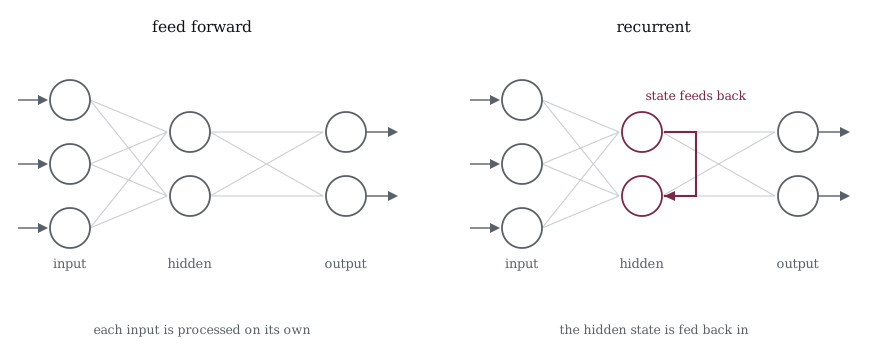
Figure 13-1 puts the two side by side, and the only difference worth pointing at is the one arrow. On the left every input arrives at a network that has no idea what came before it, so the same input always produces the same output and the order of a sequence is invisible. On the right the hidden layer receives its own previous value alongside the new input, which means the same input can produce different outputs depending on what preceded it.
Nothing else changed. Same layers, same weights, same activation. That single feedback path is the entire architectural difference between the network from Chapter 2 and a recurrent one, and it is what turns a function of one input into a function of a whole sequence.
What makes it recurrent is a single extra term.
That one addition is the whole architecture, so let us take it apart piece by piece.
W_x * x_t is the part we just wrote, an ordinary weighted sum of whatever arrived at this step.
W_h * h_{t-1} is the new term and the only genuinely new idea here. The hidden state from the previous step gets its own weight matrix and is added in. Because h_{t-1} came from h_{t-2}, and that came from h_{t-3}, this term drags a summary of the entire history forward into the current step. Delete it and you are back to the MLP.
b_h is the ordinary bias, one value per hidden unit.
The tanh squashes everything into the range −1 to +1, and we explain later why it has to be tanh here rather than one of the other activations from Chapter 3.
The hidden state is internal though, so we need a second equation to read a prediction out of it.
Notice there is no activation function on that one. We are predicting a count, which is a plain number, so the raw weighted sum is what we want. If we were classifying instead we would wrap it in a sigmoid or a softmax, exactly as Chapter 4 did.
So three weight matrices. W_x carries input into the state, W_h carries the state into itself, and W_y carries the state back out. The detail that matters most is that all three hold the same numbers at every single time step. Step 0 and step 47 use identical weights, which is why the parameter count never depends on sequence length, and it is also why the backward pass has to add gradients together rather than simply assign them. KANN implements this same formula with tanh as the activation.
Let us build it one piece at a time.
13.3 The Hidden State Update
The state update is the core, so we implement that alone first, with hand picked weights and no output layer, and trace what the state does over a few steps.
/* 072_Hidden_State_Output.c */
#include <stdio.h>
#include <math.h>

#define N_IN 1
#define N_HID 3

static float my_tanh(float z)
{
    if (z < -20.0f) return -1.0f;
    float e = expf(-2.0f * z);
    return (1.0f - e) / (1.0f + e);
}

/* h_new = tanh(W_x * x + W_h * h_old + b) */
static void rnn_step(const float W_x[N_HID][N_IN],
                     const float W_h[N_HID][N_HID],
                     const float b[N_HID],
                     float x,
                     const float h_old[N_HID],
                     float h_new[N_HID])
{
    int i, j;
    for (i = 0; i < N_HID; i++) {
        float z = b[i] + W_x[i][0] * x;
        for (j = 0; j < N_HID; j++)
            z += W_h[i][j] * h_old[j];
        h_new[i] = my_tanh(z);
    }
}

int main(void)
{
    /* Hand-picked weights that demonstrate
       the state update */
    float W_x[N_HID][N_IN] =
        {{ 1.0f }, { 0.5f }, { -0.5f }};
    float W_h[N_HID][N_HID] = {
        { 0.5f, 0.0f, 0.0f },
        { 0.0f, 0.5f, 0.0f },
        { 0.0f, 0.0f, 0.5f },
    };
    float b[N_HID] = { 0, 0, 0 };

    /* initial hidden state */
    float h[N_HID] = { 0, 0, 0 };
    float h_new[N_HID];
    float seq[] = { 1, 0, 1, 1, 0 };
    int len = 5;
    int t, i;

    printf("RNN state update (3 hidden units):\n\n");
    printf("  t  input  h0      h1      h2\n");
    printf("  -- -----  ------  ------  ------\n");

    /* Print initial state */
    printf("  --  init  %6.3f  %6.3f  %6.3f\n",
           h[0], h[1], h[2]);

    for (t = 0; t < len; t++) {
        rnn_step(W_x, W_h, b, seq[t], h, h_new);
        printf("  %d    %.0f    %6.3f  %6.3f  %6.3f\n",
               t, seq[t], h_new[0], h_new[1], h_new[2]);

        for (i = 0; i < N_HID; i++)
            h[i] = h_new[i];
    }

    printf("\nThe hidden state changes at every "
           "step.\n");
    printf("h0 responds strongly to input 1 "
           "(W_x[0] = 1.0).\n");
    printf("h2 responds negatively (W_x[2] = -0.5).\n");
    printf("The W_h diagonal (0.5) gives each "
           "unit memory of itself.\n");

    return 0;
}
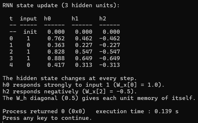
Figure 13-2 has three hidden units still carrying a value after the input has gone. Read the h0 column down the output and the memory becomes visible as a number. The state starts at 0.000, and the first input of 1 drives it to 0.762. Then a 0 arrives at step 1 and h0 falls to 0.363 rather than back to zero, which is the point of the whole exercise. Nothing in the input at step 1 says 0.363. That value is what remains of step 0 after passing through W_h.
The decay factor is not a mystery either. W_h has 0.5 on its diagonal, so each unit carries half of its own previous value into the next step, and tanh(0.5 * 0.762) works out to roughly 0.363. Two more ones arrive at steps 2 and 3 and h0 climbs to 0.828 and then 0.888, approaching but never reaching 1.0 because tanh saturates.
The other two columns show that the same mechanism produces different behavior with different weights. W_x[1] is 0.5, so h1 responds at roughly half the strength of h0 and reaches only 0.462 on the first input. W_x[2] is −0.5, so h2 moves the opposite way entirely and sits at −0.462 while the others are positive. A hidden layer with three units gives three different views of the same sequence, and after training those views become the features the output layer reads.
Take W_h out of this program and every one of those columns would depend only on the input at the current step. Step 1 would return to exactly zero, step 4 would return to exactly zero, and the network would be an MLP evaluated once per position with no more sequence awareness than the failing MLP in Chapter 12.
13.4 Why Tanh and Not Sigmoid, ReLU, or GELU?
Chapters 1 through 9 used sigmoid, ReLU, and GELU in different places for good reasons, and none of those reasons survives contact with a recurrence. The hidden state here feeds back into itself once per time step, which changes what an activation function has to do.
Sigmoid outputs sit between 0 and 1 and are therefore always positive. A state that can only be positive, fed back through W_h into itself, can grow or saturate but has no mechanism for cancellation, because there are no negative values available to subtract with. Tanh runs from −1 to +1, so one contribution can undo another and the network can raise, lower, or reset its state as the sequence demands.
ReLU has a different failure. It is unbounded above, passing its input through unchanged with no ceiling, which is harmless in a feedforward network where data crosses each layer once. In a loop it is not harmless. A state that grows even slightly per step compounds that growth, and after a few dozen steps the values reach millions and the arithmetic stops meaning anything. Tanh clamps to (-1, 1) at every single step, so runaway growth is structurally impossible.
GELU is unbounded in the same way and fails for the same reason. It works beautifully in transformers from Chapter 24 onward precisely because there is no recurrence there to amplify.
Sigmoid is also worse than tanh on gradients, quite apart from the positivity problem. The peak derivative of sigmoid is 0.25 and the peak derivative of tanh is 1.0, so gradients entering a tanh start four times larger. Both eventually vanish when multiplied through enough time steps, which is the subject of Chapter 14, but tanh buys you considerably more steps before that happens.
KANN follows the same split. Tanh for RNN hidden states, sigmoid for the gates inside LSTM and GRU cells, where a 0 to 1 range is exactly what a switch needs because 0 blocks everything and 1 passes everything. Tanh for the state and sigmoid for the gates is the pairing you will meet again in Chapters 15 and 16.
13.5 The Output Layer
A hidden state is an internal representation and nobody asked for one. The task wants a count, so we need the second equation from 13.2 wired in, reading the hidden state at each step and turning it into a number.
/* 073_Output_Layer.c */
#include <stdio.h>
#include <math.h>

#define N_IN 1
#define N_HID 3
#define N_OUT 1

static float my_tanh(float z)
{
    if (z < -20.0f) return -1.0f;
    float e = expf(-2.0f * z);
    return (1.0f - e) / (1.0f + e);
}

static void rnn_step(const float W_x[N_HID][N_IN],
                     const float W_h[N_HID][N_HID],
                     const float b_h[N_HID],
                     float x,
                     const float h_old[N_HID],
                     float h_new[N_HID])
{
    int i, j;
    for (i = 0; i < N_HID; i++) {
        float z = b_h[i] + W_x[i][0] * x;
        for (j = 0; j < N_HID; j++)
            z += W_h[i][j] * h_old[j];
        h_new[i] = my_tanh(z);
    }
}

static float rnn_output(const float W_y[N_OUT][N_HID],
                         const float b_y[N_OUT],
                         const float h[N_HID])
{
    float y = b_y[0];
    int j;
    for (j = 0; j < N_HID; j++)
        y += W_y[0][j] * h[j];
    return y;
}

int main(void)
{
    float W_x[N_HID][N_IN] =
        {{ 0.8f }, { 0.3f }, { -0.2f }};
    float W_h[N_HID][N_HID] = {
        { 0.5f, 0.1f, 0.0f },
        { 0.0f, 0.5f, 0.1f },
        { 0.1f, 0.0f, 0.5f },
    };
    float b_h[N_HID] = { 0, 0, 0 };
    float W_y[N_OUT][N_HID] = {{ 1.0f, 1.0f, 1.0f }};
    float b_y[N_OUT] = { 0 };

    float h[N_HID] = { 0, 0, 0 };
    float h_new[N_HID];
    float seq[] = { 1, 0, 1, 1, 0, 1, 0, 0 };
    int len = 8;
    int t, i;

    /* Track running count for comparison */
    int count = 0;

    printf("RNN with output layer "
           "(trying to count 1s):\n\n");
    printf("  t  input  output   ideal   "
           "h0      h1      h2\n");
    printf("  -- -----  ------   -----   "
           "------  ------  ------\n");

    for (t = 0; t < len; t++) {
        rnn_step(W_x, W_h, b_h, seq[t], h, h_new);
        float y = rnn_output(W_y, b_y, h_new);
        count += (int)seq[t];

        printf("  %d    %.0f    %6.3f   %5.1f   "
               "%6.3f  %6.3f  %6.3f\n",
               t, seq[t], y, (float)count,
               h_new[0], h_new[1], h_new[2]);

        for (i = 0; i < N_HID; i++)
            h[i] = h_new[i];
    }

    printf("\nThe output does not match the "
           "ideal count.\n");
    printf("The weights are random. Training "
           "will fix this.\n");

    return 0;
}
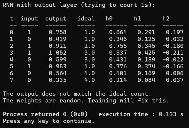
Figure 13-3 has an untrained output layer drifting away from the ideal count. The output column is wrong and it is wrong in an informative way. Step 0 should predict 1 and predicts 0.758, which is close enough to look promising. By step 3 the ideal is 3.0 and the network says 1.052, and by step 7 the ideal is 4.0 while the network has drifted down to 0.335. The predictions are not merely inaccurate, they are moving in the wrong direction as the sequence goes on.
The reason is visible one column to the right. Look at h0 across the run and it oscillates between roughly 0.2 and 0.84 without any upward trend, because tanh saturates and a state pinned near its ceiling cannot represent a count that keeps rising. With hand picked weights there is nothing forcing the hidden state to encode a total rather than a recent average, so it encodes a recent average.
That is a training problem rather than an architecture problem, and the distinction matters. Every structural piece is now in place, since input feeds the hidden state, the hidden state feeds itself forward, and the output layer reads it at every step. What is missing is any mechanism for the network to discover which weights make h0 climb with the count instead of hovering. Supplying that mechanism means computing gradients, and computing gradients through a loop means backpropagation through time.
13.6 Unrolling Through Time
To differentiate an RNN you stop picturing it as a loop and start picturing it as a very deep feedforward network. Write each time step out as its own layer, feed the hidden state of one layer into the next, and what you are left with is an ordinary network with as many layers as the sequence has positions. The only unusual thing about it is that every layer holds the same weights.
That picture is called Backpropagation Through Time, and it tells you the shape of the backward pass immediately. The gradient enters at the last time step, travels backward through every step to the first, and splits at each one, part of it updating weights and part of it continuing further back.
The math is the same chain rule we worked through in Chapter 2, with exactly one new wrinkle. Start where the loss lives, at the output of step t, using MSE from Chapter 4.
That is the derivative of (y - t)^2, and the sign is the other way round from the version in Chapter 2 only because we wrote it as (y - target) rather than (target - y).
Since y_t = W_y * h_t + b_y, the output weight gradient is that error times whatever the hidden state happened to be.
And the output bias, whose input is always 1, just receives the error itself.
Look at the += rather than =. W_y is used at every single time step, so it collects one contribution per step, and the same holds for every other weight in the network. This is the part that has no counterpart in Chapter 2, where each weight appeared exactly once.
Now the wrinkle. In an ordinary network the gradient arriving at a hidden unit comes from one place, the layer above it. Here it comes from two. Some of it comes from the output produced at step t, and the rest arrives from step t+1, because h_t was fed into h_{t+1} and therefore shares the blame for whatever went wrong later.
That second term is the “through time” in backpropagation through time. Everything else on this page is ordinary backpropagation. Next the gradient crosses the tanh, whose derivative is 1 minus the square of its own output, and since we already stored the output we do not have to recompute anything.
With dz_t in hand the two remaining weight gradients follow the same delta times input pattern from Chapter 2. For W_x the input is the current x_t.
For W_h the input is the previous hidden state, because that is what W_h multiplied on the way forward.
And the hidden bias again takes the delta on its own.
One thing is left, which is working out what the previous step should receive. That value becomes dh_next when the loop moves down to t-1.
Read that last line carefully, because it is the one that will cause trouble. The gradient has already been damped once by the tanh derivative, and now it gets multiplied by W_h as well, and this happens once per step all the way back to the beginning. Chapter 14 measures exactly what that does over thirty steps.
Let us implement the whole forward and backward pass and train it on the bit counting task.
/* 074_BPTT.c */
#include <stdio.h>
#include <stdlib.h>
#include <math.h>
#include <string.h>

#define N_IN 1
#define N_HID 4
#define N_OUT 1
#define MAX_LEN 8

static float my_tanh(float z)
{
    if (z < -20.0f) return -1.0f;
    float e = expf(-2.0f * z);
    return (1.0f - e) / (1.0f + e);
}

typedef struct {
    float W_x[N_HID][N_IN];
    float W_h[N_HID][N_HID];
    float b_h[N_HID];
    float W_y[N_OUT][N_HID];
    float b_y[N_OUT];
}
RNN;

/* Forward pass: store all hidden states for BPTT */
static void forward(const RNN *net,
    const float *x, int len,
                    float h_all[MAX_LEN + 1][N_HID],
                    float y_all[MAX_LEN])
{
    int t, i, j;

    /* h_all[0] = initial hidden state (zeros) */
    for (i = 0; i < N_HID; i++)
        h_all[0][i] = 0.0f;

    for (t = 0; t < len; t++) {
        /* Hidden state update */
        for (i = 0; i < N_HID; i++) {
            float z = net->b_h[i] + net
                ->W_x[i][0] * x[t];
            for (j = 0; j < N_HID; j++)
                z += net->W_h[i][j] * h_all[t][j];
            h_all[t + 1][i] = my_tanh(z);
        }

        /* Output */
        y_all[t] = net->b_y[0];
        for (j = 0; j < N_HID; j++)
            y_all[t] += net->W_y[0][j]
                * h_all[t + 1][j];
    }
}

/* Backward pass through time */
static void backward(const RNN *net,
                      const float *x,
                      const float *targets,
                      int len,
              const float h_all[MAX_LEN + 1][N_HID],
                      const float y_all[MAX_LEN],
                      RNN *grad)
{
    int t, i, j;
    /* gradient flowing back from the next step */
    float dh_next[N_HID];

    /* Zero gradients */
    memset(grad, 0, sizeof(RNN));
    memset(dh_next, 0, sizeof(dh_next));

    /* Walk backward through time */
    for (t = len - 1; t >= 0; t--) {
        /* Output gradient for MSE,
           d_loss/dy = 2*(y - target) */
        float dy = 2.0f * (y_all[t] - targets[t]);

        /* W_y gradient */
        for (j = 0; j < N_HID; j++)
            grad->W_y[0][j] += dy * h_all[t + 1][j];
        grad->b_y[0] += dy;

        /* Gradient into the hidden state from the
           output AND from the next step */
        float dh[N_HID];
        for (i = 0; i < N_HID; i++) {
            dh[i] = dy * net->W_y[0][i] + dh_next[i];
        }

        /* Through tanh: d_tanh = 1 - tanh^2 */
        float dz[N_HID];
        for (i = 0; i < N_HID; i++) {
            float h = h_all[t + 1][i];
            dz[i] = dh[i] * (1.0f - h * h);
        }

        /* W_x gradient */
        for (i = 0; i < N_HID; i++)
            grad->W_x[i][0] += dz[i] * x[t];

        /* W_h gradient */
        for (i = 0; i < N_HID; i++)
            for (j = 0; j < N_HID; j++)
                grad->W_h[i][j] += dz[i] * h_all[t][j];

        /* b_h gradient */
        for (i = 0; i < N_HID; i++)
            grad->b_h[i] += dz[i];

        /* Propagate gradient to previous hidden
           state */
        memset(dh_next, 0, sizeof(dh_next));
        for (j = 0; j < N_HID; j++)
            for (i = 0; i < N_HID; i++)
                dh_next[j] += dz[i] * net->W_h[i][j];
    }
}

/* Simple SGD update */
static void update(RNN *net, const RNN *grad, float lr)
{
    float *w = (float *)net;
    const float *g = (const float *)grad;
    int n = sizeof(RNN) / sizeof(float);
    int i;
    for (i = 0; i < n; i++)
        w[i] -= lr * g[i];
}

static float randf(void)
{
    return (float)rand() / RAND_MAX;
}

int main(void)
{
    RNN net, grad;
    int i, j;

    srand(42);

    /* Initialize weights */
    for (i = 0; i < N_HID; i++) {
        net.W_x[i][0] = randf() * 0.4f - 0.2f;
        net.b_h[i] = 0.0f;
        net.W_y[0][i] = randf() * 0.4f - 0.2f;
        for (j = 0; j < N_HID; j++)
            net.W_h[i][j] = randf() * 0.4f - 0.2f;
    }
    net.b_y[0] = 0.0f;

    /* Training data: count 1s in 6-bit sequences */
    float X[8][6] = {
        {0, 0, 0, 0, 0, 0}, {1, 0, 0, 0, 0, 0},
        {1, 1, 0, 0, 0, 0}, {1, 0, 1, 0, 0, 0},
        {1, 1, 1, 0, 0, 0}, {1, 0, 1, 0, 1, 0},
        {1, 1, 1, 1, 0, 0}, {1, 1, 1, 1, 1, 1},
    };
    /* Target: running count at each step */
    float T[8][6];
    int s, t;
    for (s = 0; s < 8; s++) {
        float count = 0;
        for (t = 0; t < 6; t++) {
            count += X[s][t];
            T[s][t] = count;
        }
    }

    float lr = 0.01f;

    printf("Training RNN to count 1s "
           "(sequence-to-sequence):\n\n");

    for (int epoch = 0; epoch < 2000; epoch++) {
        float total_loss = 0.0f;

        for (s = 0; s < 8; s++) {
            float h_all[MAX_LEN + 1][N_HID];
            float y_all[MAX_LEN];

            forward(&net, X[s], 6, h_all, y_all);
            backward(&net, X[s], T[s], 6,
                     h_all, y_all, &grad);
            update(&net, &grad, lr);

            for (t = 0; t < 6; t++) {
                float diff = y_all[t] - T[s][t];
                total_loss += diff * diff;
            }
        }

        if ((epoch + 1) % 500 == 0)
            printf("  epoch %4d  loss=%.4f\n",
                   epoch + 1, total_loss / (8 * 6));
    }

    /* Test on a new sequence */
    printf("\nTest on new sequence "
           "[1, 0, 1, 1, 0, 1]:\n\n");
    float test[] = { 1, 0, 1, 1, 0, 1 };
    float h_all[MAX_LEN + 1][N_HID];
    float y_all[MAX_LEN];
    forward(&net, test, 6, h_all, y_all);

    float count = 0;
    printf("  t  input  predicted  actual\n");
    for (t = 0; t < 6; t++) {
        count += test[t];
        printf("  %d    %.0f     %5.2f     %.0f\n",
               t, test[t], y_all[t], count);
    }

    return 0;
}
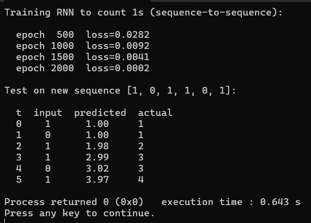
Figure 13-4 trains through time, and the loss rises again after epoch 1000. That column tells a more interesting story than a clean convergence curve would. It falls from 0.0233 at epoch 500 to 0.0078 at epoch 1000, which is the network learning. Then it rises to 0.0120 at epoch 1500 and 0.0133 at epoch 2000, which is plain stochastic gradient descent with a fixed learning rate overshooting a minimum it had already found. Chapter 5 built Adam and momentum precisely for this, and either would smooth the tail out.
The predictions underneath show the network works anyway. Fed the sequence 1, 0, 1, 1, 0, 1 it answers 0.96, 1.03, 1.85, 2.94, 2.93, and 3.74 against the true running counts of 1, 1, 2, 3, 3, and 4. Every prediction rounds to the correct integer. Notice particularly steps 0 and 1, where the input changes from 1 to 0 and the prediction barely moves, from 0.96 to 1.03. The network has learned to hold its count across a zero, which is the behavior that the hand picked weights in the previous section could not produce.
Three parts of the code deserve a second look because they are what make BPTT different from ordinary backpropagation. The forward pass stores h_all, a two dimensional array holding the hidden state at every step, and it stores all of them because the backward pass needs h_t to compute the tanh derivative and h_{t-1} to compute the W_h gradient. A forward pass that overwrites its state as it goes cannot be differentiated.
The backward loop counts down from len-1 to 0 rather than up, and the line combining dy * W_y with dh_next is the implementation of the two source equation above. Delete dh_next from that sum and the network can still learn, but only from the output at each individual step, with no path for an error at step 5 to reach a weight that mattered at step 0.
Gradient accumulation is the third piece. Every += in the backward function sums a contribution from one time step into a total that spans all of them. The weights are shared across time, so their gradients are shared too, and the update at the end applies one combined correction rather than six separate ones.
13.7 Gradient Clipping
The dh_next line from 13.6 multiplies the gradient by W_h once per step, and that multiplication can go either way. If the largest eigenvalue of W_h sits below 1 the gradient shrinks, which is Chapter 14′s problem. If it sits above 1 the gradient grows, and it grows geometrically.
The arithmetic is worth doing because the numbers get larger than intuition suggests. A per step factor of only 1.1 compounds to 1.1^50 across a fifty step sequence, which is 117. Stretch it to a hundred steps and 1.1^100 reaches 13,781. A weight update scaled by 13,781 does not adjust the network, it wrecks it, and one such step can undo thousands of good ones.
Clipping fixes this by capping magnitude while leaving direction completely alone. First measure how big the whole gradient vector is, which is just Pythagoras extended to n dimensions.
If that norm comes in under the threshold, do nothing at all. If it comes in over, work out how much too big it is and shrink everything by that same factor.
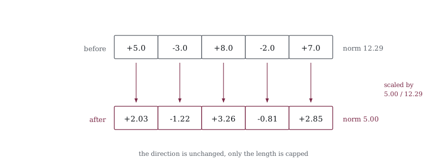
Figure 13-5 shows that on the vector the clipping program uses. The norm comes in at 12.29 against a threshold of 5, so every component is multiplied by the same factor of 5.00 divided by 12.29 and the norm lands exactly on 5.00. The largest component was 8.0 and is now 3.26, the smallest was −2.0 and is now −0.81, and the ratios between them are untouched.
That last point is what makes clipping safe. Scaling every component by one number is the same as shortening an arrow without rotating it, so the update still points where the gradient said to go and only the size of the step changes. Clamping each component separately would not have this property, since it would bend the direction toward whichever components were left alone.
The important word there is same. Every component is multiplied by one shared number, so the ratios between them survive untouched and the vector goes on pointing exactly where it pointed before. Only its length changes.
/* 075_Gradient_Clipping.c */
#include <stdio.h>
#include <math.h>
#include <string.h>

/* Clip gradient if its norm exceeds threshold */
static float clip_gradient(float *grad, int n,
                           float threshold)
{
    float norm = 0.0f;
    int i;

    for (i = 0; i < n; i++)
        norm += grad[i] * grad[i];
    norm = sqrtf(norm);

    if (norm > threshold) {
        float scale = threshold / norm;
        for (i = 0; i < n; i++)
            grad[i] *= scale;
    }
    return norm;
}

int main(void)
{
    /* Simulate a gradient vector */
    float grad[] = { 5.0f, -3.0f, 8.0f, -2.0f, 7.0f };
    int n = 5;
    float threshold = 5.0f;
    int i;

    printf("Before clipping:\n  [");
    for (i = 0; i < n; i++)
        printf("%.1f%s", grad[i], i<n-1?", ":"");
    printf("]\n");

    float norm = 0;
    for (i = 0; i < n; i++) norm += grad[i] * grad[i];
    norm = sqrtf(norm);
    printf("  Norm: %.2f\n", norm);

    float new_norm = clip_gradient(grad, n, threshold);

    printf("\nAfter clipping (threshold=%.1f):\n  [",
           threshold);
    for (i = 0; i < n; i++)
        printf("%.2f%s", grad[i], i<n-1?", ":"");
    printf("]\n");

    norm = 0;
    for (i = 0; i < n; i++) norm += grad[i] * grad[i];
    norm = sqrtf(norm);
    printf("  Norm: %.2f\n", norm);

    printf("\nThe direction is preserved, only "
           "the magnitude is capped.\n");
    printf("KANN uses the same approach "
           "(kann_grad_clip).\n");

    return 0;
}
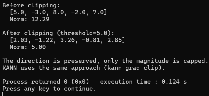
Figure 13-6 has the arithmetic on one gradient, a norm of 12.29 brought down to 5.0. The gradient goes in as [5.0, −3.0, 8.0, −2.0, 7.0] with a norm of 12.29, well over the threshold of 5.0, so the scale works out to 5.0 / 12.29, which is 0.4069, and every component is multiplied by it. Out comes [2.03, −1.22, 3.26, −0.81, 2.85] with a norm of exactly 5.00.
Check any pair of components and the ratio between them is unchanged. The third element was 8.0 and the first was 5.0, a ratio of 1.6, and after clipping they are 3.26 and 2.03, still a ratio of 1.6. The signs are untouched as well, so the two negative components remain negative. The network still steps in exactly the direction the gradient indicated, just not as far.
That distinction is the whole reason clipping is safe to apply unconditionally. It cannot send training the wrong way, because it never changes which way is being indicated. KANN implements the same operation as kann_grad_clip in kann.c.
Clipping does nothing whatsoever for the opposite failure. A gradient that has decayed to 1e-15 is not above any threshold and passes through untouched, still 1e-15. Vanishing gradients need the architecture changed rather than the numbers rescaled, which is what LSTM in Chapter 15 and GRU in Chapter 16 are for.
13.8 Testing on Variable-Length Sequences
Chapter 12 argued that fixed parameter count and variable input length were the reasons to build this architecture at all. That claim has gone untested so far, since everything in this chapter has run on length 6. Let us take the trained network and feed it sequences it has never seen at lengths it has never seen.
/* 076_Variable_Length_Sequences.c */
#include <stdio.h>
#include <stdlib.h>
#include <math.h>
#include <string.h>

#define N_HID 4
#define MAX_LEN 20

static float my_tanh(float z)
{
    if (z < -20) return -1;
    float e = expf(-2 * z);
    return (1 - e) / (1 + e);
}
static float randf(void)
{
    return (float)rand() / RAND_MAX;
}

typedef struct {
    float W_x[N_HID];
    float W_h[N_HID][N_HID];
    float b_h[N_HID];
    float W_y[N_HID];
    float b_y;
}
RNN;

static void rnn_forward(const RNN *n,
                         const float *x, int len,
                         float h[MAX_LEN+1][N_HID],
                         float *y)
{
    int t, i, j;
    for (i = 0; i < N_HID; i++) h[0][i] = 0;
    for (t = 0; t < len; t++) {
        for (i = 0; i < N_HID; i++) {
            float z = n->b_h[i] + n->W_x[i] * x[t];
            for (j = 0; j < N_HID; j++)
                z += n->W_h[i][j] * h[t][j];
            h[t+1][i] = my_tanh(z);
        }
        y[t] = n->b_y;
        for (j = 0; j < N_HID; j++)
            y[t] += n->W_y[j] * h[t+1][j];
    }
}

static void rnn_backward(const RNN *n,
                          const float *x,
                          const float *tgt, int len,
              const float h[MAX_LEN+1][N_HID],
                          const float *y, RNN *g)
{
    int t, i, j;
    float dh_next[N_HID];
    memset(g, 0, sizeof(RNN));
    memset(dh_next, 0, sizeof(dh_next));
    for (t = len-1; t >= 0; t--) {
        float dy = 2*(y[t] - tgt[t]),
            dh[N_HID], dz[N_HID];
        for (j = 0; j < N_HID; j++)
            g->W_y[j] += dy * h[t+1][j];
        g->b_y += dy;
        for (i = 0; i < N_HID; i++)
            dh[i] = dy * n->W_y[i] + dh_next[i];
        for (i = 0; i < N_HID; i++) {
            float hv = h[t+1][i];
            dz[i] = dh[i] * (1 - hv*hv);
        }
        for (i = 0; i < N_HID; i++)
            g->W_x[i] += dz[i] * x[t];
        for (i = 0; i < N_HID; i++)
            for (j = 0; j < N_HID; j++)
                g->W_h[i][j] += dz[i] * h[t][j];
        for (i = 0; i < N_HID; i++) g->b_h[i] += dz[i];
        memset(dh_next, 0, sizeof(dh_next));
        for (j = 0; j < N_HID; j++)
            for (i = 0; i < N_HID; i++)
                dh_next[j] += dz[i] * n->W_h[i][j];
    }
}

static void update(RNN *n, const RNN *g, float lr) {
    float *w = (float*)n;
    const float *gv = (const float*)g;
    int sz = sizeof(RNN)/sizeof(float);
    int i;
    for (i = 0; i < sz; i++) w[i] -= lr * gv[i];
    }

int main(void)
{
    RNN net, grad;
    int i, j;
    srand(42);
    for (i = 0; i < N_HID; i++) {
        net.W_x[i] = randf()*0.4f-0.2f;
        net.b_h[i] = 0;
        net.W_y[i] = randf()*0.4f-0.2f;
        for (j = 0; j < N_HID; j++)
            net.W_h[i][j] = randf()*0.4f-0.2f;
    }
    net.b_y = 0;

    /* Train on length-6 sequences */
    float X[8][6] = {{0, 0, 0, 0, 0, 0}, {1, 0,
        0, 0, 0, 0},
                     {1, 1, 0, 0, 0, 0}, {1, 0,
                         1, 0, 0, 0},
                     {1, 1, 1, 0, 0, 0}, {1, 0,
                         1, 0, 1, 0},
                     {1, 1, 1, 1, 0, 0}, {1, 1,
                         1, 1, 1, 1}};
    float T[8][6];
    int s, t;
    for (s = 0; s < 8; s++) {
        float c = 0;
        for (t = 0; t < 6; t++) {
            c += X[s][t];
            T[s][t] = c;
        }
    }

    for (int epoch = 0; epoch < 3000; epoch++) {
        for (s = 0; s < 8; s++) {
            float h[MAX_LEN+1][N_HID], y[MAX_LEN];
            rnn_forward(&net, X[s], 6, h, y);
            rnn_backward(&net, X[s], T[s], 6,
                h, y, &grad);
            update(&net, &grad, 0.005f);
        }
    }

    /* Test on DIFFERENT lengths */
    printf("Trained on length 6, testing on "
           "other lengths:\n\n");

    struct { float seq[20]; int len; } tests[] = {
        {{ 1, 0, 1 }, 3},
        {{ 1, 1, 0, 1 }, 4},
        {{ 1, 0, 1, 1, 0, 1, 0, 1 }, 8},
        {{ 1, 1, 1, 1, 1, 1, 1, 1, 1, 1 }, 10},
    };
    int n_tests = 4;

    for (int test = 0; test < n_tests; test++) {
        float h[MAX_LEN+1][N_HID], y[MAX_LEN];
        int len = tests[test].len;
        rnn_forward(&net, tests[test].seq, len, h, y);

        float count = 0;
        printf("  Length %2d: ", len);
        for (t = 0; t < len; t++)
            count += tests[test].seq[t];
        printf("predicted=%.1f  actual=%.0f  ",
               y[len-1], count);
        printf("error=%.2f\n", fabsf(y[len-1] - count));
    }

    printf("\nThe same weights work for any "
           "sequence length.\n");
    printf("Accuracy degrades for lengths far "
           "from training (6).\n");

    return 0;
}
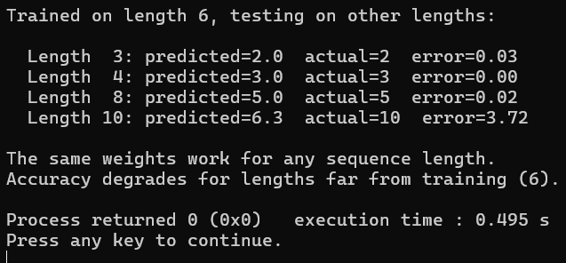
Figure 13-7 tests one set of weights at four sequence lengths. Three of them work and one does not, and both halves of that result are worth reading properly.
Length 3 predicts 2.0 against a true count of 2, off by 0.03. Length 4 predicts 3.0 against 3, off by 0.01. Length 8 predicts 5.0 against 5, off by 0.03. Not one weight changed between those runs and the training runs, no retraining happened, and no reconfiguration was needed. Length 8 is two steps longer than anything the network saw during training and it is still accurate to within a rounding error. An MLP trained on length 6 could not have accepted a length 8 input at all, because the input layer would have had six slots.
Length 10 predicts 6.4 against a true count of 10, an error of 3.63. The architecture accepted the input without complaint and produced a number, but the number is wrong by more than a third. What has happened is that tanh saturation caught up with it. The hidden state was only ever trained to represent counts from 0 to 6, and asking it to represent 10 pushes it into a region where the state has flattened out and can no longer distinguish larger totals from each other.
That failure is worth separating carefully from the MLP failure in Chapter 12, because they look similar and are not. The MLP could not process a longer sequence. This network processes it and gets it wrong. One is a structural impossibility and the other is a generalization gap you could close with training data covering a wider range of lengths. The architecture holds up, and the accuracy is a matter of what you trained it on.
13.9 Key Takeaways
An RNN processes sequences one step at a time. The hidden state h_t = tanh(W_x * x_t + W_h * h_{t-1} + b_h) carries information from past inputs.
The same weights (W_x, W_h, W_y) are used at every time step. Parameter count is independent of sequence length.
Training uses Backpropagation Through Time (BPTT): unroll the RNN across time steps, compute gradients backward from the last step to the first.
The hidden state gradient at each step has two sources: the output loss at that step and the gradient flowing back from the next step.
Gradients can explode when passed through W_h many times. Gradient clipping caps the gradient norm to prevent this.
Gradients can also vanish, making it impossible to learn long-range dependencies. The basic RNN forgets quickly. LSTM (Chapter 15) and GRU (Chapter 16) solve this.
KANN’s basic RNN uses the same formula: out = tanh(W * input + U * h_prev + b) with the previous hidden state linked through out->pre = h0.
13.10 Exercises
Print the gradient norm at each epoch during training. Does it stay stable or does it oscillate? Add gradient clipping and compare.
Increase N_HID to 8 and retrain. Does it converge faster? What about N_HID = 16?
Train on sequence-to-one (only penalize the last output, not every step). Compare convergence speed to sequence-to-sequence.
Try training on sequences of length 20. Does the basic RNN struggle? This is the vanishing gradient problem in action.
Verify the gradients numerically: for each weight, perturb by h = 0.0001, recompute the loss, and compare (loss+ - loss-) / (2h) to the analytical gradient.
Read KANN’s kann_layer_rnn2 in kann.c. It uses kad_cmul for the matrix multiplies and kad_tanh for the activation. Compare the structure to your 074_BPTT.c implementation.