Query/Key/Value Attention
Learnable version of dot-product attention
20.1 What You Will Learn
Chapter 19 built attention out of the encoder states themselves, using each state both as the thing the query is compared against and as the thing that gets retrieved. That works, and it was the right way to meet the mechanism, but it quietly imposes a constraint. Deciding whether a position is relevant and deciding what that position should contribute are different questions, and forcing one vector to answer both means the answers cannot be tuned independently.
This chapter removes the constraint with three learned matrices. Each input is projected into a query, a key and a value, so a position can be matched on one aspect of itself and retrieved for another. Nothing about the attention arithmetic changes, since it is still score, normalize and blend. What changes is that the network now chooses what goes into each of the three slots rather than being handed the raw embedding for all three.
We build the projections first, then run them over a sequence so every position attends to every other, then construct a case where the projections produce an attention pattern the raw vectors could never produce. At the end of the chapter we package the whole thing into one function, which is the exact block that appears inside every transformer layer from Chapter 24 onward.
20.2 The Limitation of Raw Dot Product
The attention from Chapter 19 scored a decoder state against encoder states directly and then blended those same encoder states.
The encoder state appears twice in those two lines, once as the thing compared and once as the thing retrieved, and that double duty is the limitation. Take the word bank. To decide whether it is relevant to what the decoder is currently producing, the useful signal might be whether this occurrence means money or a river. To decide what bank should contribute once selected, the useful signal might be its grammatical role or its translation. Those are different facts about the same word, and a single vector has to encode both while also being the thing the similarity is computed on.
The problem is sharper than it sounds because similarity in embedding space is fixed before attention ever runs. Two words with similar embeddings will always score highly against each other, whatever the task wants. A model that needs a determiner to attend to its noun, or a verb to attend to its subject, has no way to express that if determiners and nouns happen to sit far apart in embedding space. The geometry of the input decides the attention pattern, and the network gets no say.
20.3 Separate Projections
Three matrices fix it. W_Q, W_K and W_V each multiply the input and produce a different vector, so one embedding becomes three representations with three jobs.
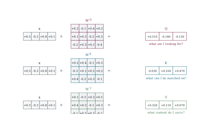
Figure 20-1 works those three lines through with the numbers the first program in this chapter uses. The same four value input appears on every row, and the only thing that differs is the matrix it passes through, so the three results have nothing in common beyond where they came from.
The shapes matter as much as the values. The input is four dimensional and all three outputs are three dimensional, which means the projections are free to change the size of the space as well as its orientation. Q and K only ever meet in a dot product, so they must match each other, while V is never compared against anything and can be any width the model finds useful.
Q is what this position is looking for, K is what it offers to be matched on, and V is what it contributes if selected. All three are learned, so the network decides what each one should contain.
/* 106_Projections.c */
#include <stdio.h>

#define D_MODEL 4   /* input dimension */
#define D_K 3        /* key/query dimension */
#define D_V 3        /* value dimension */

/* Matrix multiply: out[i] = sum(W[i][j] * x[j]) */
static void project(const float *x,
                    const float W[][D_MODEL],
                     float *out, int out_dim)
{
    int i, j;
    for (i = 0; i < out_dim; i++) {
        out[i] = 0;
        for (j = 0; j < D_MODEL; j++)
            out[i] += W[i][j] * x[j];
    }
}

int main(void)
{
    /* An input vector (e.g., one position's
       embedding) */
    float x[D_MODEL] = { 0.5f, -0.2f, 0.8f, 0.1f };

    /* Three learned projection matrices */
    float W_Q[D_K][D_MODEL] = {
        { 0.3f, -0.1f, 0.4f, 0.2f },
        { 0.1f, 0.5f, -0.2f, 0.3f },
        { -0.2f, 0.3f, 0.1f, -0.4f },
    };
    float W_K[D_K][D_MODEL] = {
        { 0.2f, 0.4f, -0.1f, 0.3f },
        { -0.3f, 0.1f, 0.5f, 0.2f },
        { 0.4f, -0.2f, 0.3f, -0.1f },
    };
    float W_V[D_V][D_MODEL] = {
        { 0.1f, -0.3f, 0.2f, 0.5f },
        { 0.4f, 0.2f, -0.1f, 0.3f },
        { -0.1f, 0.5f, 0.3f, -0.2f },
    };

    float q[D_K], k[D_K], v[D_V];

    project(x, W_Q, q, D_K);
    project(x, W_K, k, D_K);
    project(x, W_V, v, D_V);

    printf("Input x = [%.1f, %.1f, %.1f, %.1f]\n\n",
           x[0], x[1], x[2], x[3]);
    printf("Projected through three different "
           "matrices:\n");
    printf("  Query Q = [%+.3f, %+.3f, %+.3f]\n",
           q[0], q[1], q[2]);
    printf("  Key   K = [%+.3f, %+.3f, %+.3f]\n",
           k[0], k[1], k[2]);
    printf("  Value V = [%+.3f, %+.3f, %+.3f]\n\n",
           v[0], v[1], v[2]);

    printf("Same input, three different "
           "representations.\n");
    printf("Q asks 'what am I looking for?'\n");
    printf("K answers 'what can I be matched on?'\n");
    printf("V holds 'what content do I provide?'\n");

    return 0;
}
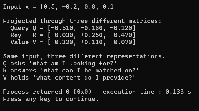
Figure 20-2 puts that one input through all three matrices. One input of [0.5, −0.2, 0.8, 0.1] produces three quite different vectors. The query is [+0.510, −0.180, −0.120], the key is [−0.030, +0.250, +0.470] and the value is [+0.320, +0.110, +0.070].
Compare the query against the key and notice they barely resemble each other. The query’s first component is +0.510 while the key’s is −0.030, and the signs disagree on the third component too. That divergence is the entire point, since if the projections produced similar vectors they would be doing the same job and two of the three matrices would be wasted. A trained network pulls them apart precisely because it needs them to carry different information.
Notice also that the projections reduce the dimension here, taking four numbers in and producing three. That is normal rather than incidental. In a transformer the query and key dimension is typically the model dimension divided by the number of attention heads, so with 512 dimensions and eight heads each head works in 64, and Chapter 21 explains why that division is the right trade.
20.4 Q/K/V Attention on a Sequence
Applied to a whole sequence, every position produces its own query, its own key and its own value from the same three matrices. Each query is then scored against every key, including the position’s own, so the result is one attention distribution per position.
The projections below are chosen rather than trained. A randomly initialized set produces near uniform weights, which demonstrates that the arithmetic runs and hides what the mechanism is for, so the numbers here were picked to make the pattern legible.
/* 107_Qkv_Sequence.c */
#include <stdio.h>
#include <math.h>

#define SEQ_LEN 4
#define D_MODEL 4
#define D_K 3

static void softmax(float *x, int n)
{
    float mx = x[0], s = 0;
    int i;
    for (i = 1; i < n; i++) if (x[i] > mx) mx = x[i];
    for (i = 0; i < n; i++) {
        x[i] = expf(x[i] - mx);
        s += x[i];
    }
    for (i = 0; i < n; i++) x[i] /= s;
}

/* out = W * x, with W stored as d_out rows of d_in */
static void project(const float W[D_K][D_MODEL],
                    const float x[D_MODEL],
                    float out[D_K])
{
    int i, j;
    for (i = 0; i < D_K; i++) {
        out[i] = 0;
        for (j = 0; j < D_MODEL; j++)
            out[i] += W[i][j] * x[j];
    }
}

int main(void)
{
    float X[SEQ_LEN][D_MODEL] = {
        {  1.0f,  0.0f,  0.5f, -0.2f },   /* the  */
        {  0.3f,  0.8f, -0.1f,  0.6f },   /* cat  */
        { -0.2f,  0.1f,  0.9f,  0.3f },   /* sat  */
        {  0.5f, -0.3f,  0.2f,  0.7f },   /* down */
    };
    const char *words[SEQ_LEN] = {
        "the", "cat", "sat", "down"
    };

    /* Chosen rather than trained, so the pattern is
       readable. Training would find its own. */
    float W_Q[D_K][D_MODEL] = {
        { -0.54f, +0.23f, +1.14f, +0.16f },
        { +1.01f, +0.59f, +3.72f, -0.67f },
        { +1.27f, +0.30f, -1.02f, +3.80f },
    };
    float W_K[D_K][D_MODEL] = {
        { +0.92f, -0.40f, +0.21f, +0.11f },
        { +0.16f, +0.92f, -0.18f, +0.33f },
        { -0.26f, -0.38f, +0.83f, +0.78f },
    };

    float Q[SEQ_LEN][D_K], K[SEQ_LEN][D_K];
    float w[SEQ_LEN];
    int i, j, k, best;

    for (i = 0; i < SEQ_LEN; i++) {
        project(W_Q, X[i], Q[i]);
        project(W_K, X[i], K[i]);
    }

    printf("Q/K/V attention on a 4 word sequence\n\n");
    for (i = 0; i < SEQ_LEN; i++) {
        for (j = 0; j < SEQ_LEN; j++) {
            w[j] = 0;
            for (k = 0; k < D_K; k++)
                w[j] += Q[i][k] * K[j][k];
        }
        softmax(w, SEQ_LEN);

        best = 0;
        for (j = 1; j < SEQ_LEN; j++)
            if (w[j] > w[best]) best = j;

        printf("  \"%-4s\" attends to: ", words[i]);
        for (j = 0; j < SEQ_LEN; j++)
            printf("%s=%.2f ", words[j], w[j]);
        printf("\n      strongest: \"%s\"\n\n",
               words[best]);
    }

    printf("Every position builds its own query, so\n");
    printf("every row differs. W_Q and W_K are\n");
    printf("shared across positions, so it is the\n");
    printf("input that differs, not the weights.\n");

    return 0;
}
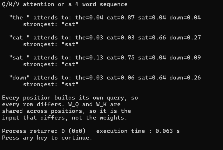
Figure 20-3 gives one attention row per position. Four positions, four different distributions, and the pattern reads like a dependency parse. The word “the” puts 0.87 on “cat”, which is the noun it determines and the only thing a determiner really relates to. The word “sat” puts 0.75 on “cat”, its subject, with a further 0.13 on “the”. Both “cat” and “down” look forward and back to “sat”, at 0.66 and 0.64 respectively, with each also keeping about a quarter of its weight on the other.
The important structural fact is that W_Q and W_K are the same matrices for all four positions. Nothing is per position and nothing is per word. The rows differ only because the inputs differ, which is what makes attention work on sequences of any length with a fixed parameter count, exactly as the shared recurrent weights did in Chapter 13.
Every position also attends to itself, since its own key is in the comparison. Here the self weights are small, 0.04 for “the” and 0.26 for “down”, but nothing forces that. A position carrying self sufficient meaning can learn to attend mostly to itself, which exercise 6 asks you to look for.
This is self-attention, so called because the queries, keys and values all come from one sequence. Cross-attention takes the queries from one sequence and the keys and values from another, which is exactly the seq2seq attention of Chapter 19 written in this notation. The arithmetic is identical and only the source of the inputs differs.
20.5 Why Separate Q, K, V Matters
The claim so far is that projections buy freedom. This section tests it by taking three words where two have deliberately similar embeddings, running attention with and without projections, and comparing the patterns.
/* 108_Why_Qkv.c */
#include <stdio.h>
#include <math.h>
#include <float.h>

#define N 3
#define D 4

static float dot(const float *a, const float *b, int n)
{
    float s = 0;
    int i;
    for (i = 0; i < n; i++) s += a[i] * b[i];
    return s;
}

static void softmax(float *x, int n)
{
    float mx = -FLT_MAX, s = 0;
    int i;
    for (i = 0; i < n; i++) if (x[i] > mx) mx = x[i];
    for (i = 0; i < n; i++) {
        x[i] = expf(x[i] - mx);
        s += x[i];
    }
    for (i = 0; i < n; i++) x[i] /= s;
}

int main(void)
{
    /* Three vectors that are geometrically similar but
       semantically different */
    float X[N][D] = {
        { 0.9f, 0.1f, 0.8f, 0.2f },   /* word A */
        /* word B, similar to A */
        { 0.8f, 0.2f, 0.7f, 0.3f },
        /* word C, different */
        { 0.1f, 0.9f, 0.2f, 0.8f },
    };

    printf("Raw dot-product attention, "
           "no projections\n\n");
    int i, j;
    for (i = 0; i < N; i++) {
        float scores[N];
        for (j = 0; j < N; j++)
            scores[j] = dot(X[i], X[j], D);
        softmax(scores, N);
        printf("  Word %c attends to: "
               "A=%.3f  B=%.3f  C=%.3f\n",
               'A' + i, scores[0],
                   scores[1], scores[2]);
    }

    printf("\nA and B always attend to each other, "
           "being similar.\n");
    printf("The network cannot learn a different "
           "pattern.\n\n");

    /* With projections, A can attend to C */
    printf("With learned Q/K projections:\n\n");

    /* W_Q designed so A's query aligns with C's key */
    float W_Q[D][D] = {
        { 0, 0, 0, 1 },
        { 0, 0, 1, 0 },
        { 0, 1, 0, 0 },
        { 1, 0, 0, 0 },
    };
    /* W_K = identity (keys unchanged) */
    float W_K[D][D] = {
        { 1, 0, 0, 0 },
        { 0, 1, 0, 0 },
        { 0, 0, 1, 0 },
        { 0, 0, 0, 1 },
    };

    float Q[N][D], K[N][D];
    for (i = 0; i < N; i++) {
        for (j = 0; j < D; j++) {
            Q[i][j] = 0;
            K[i][j] = 0;
            int k;
            for (k = 0; k < D; k++) {
                Q[i][j] += W_Q[j][k] * X[i][k];
                K[i][j] += W_K[j][k] * X[i][k];
            }
        }
    }

    for (i = 0; i < N; i++) {
        float scores[N];
        for (j = 0; j < N; j++)
            scores[j] = dot(Q[i], K[j], D);
        softmax(scores, N);
        printf("  Word %c attends to: "
               "A=%.3f  B=%.3f  C=%.3f\n",
               'A' + i, scores[0],
                   scores[1], scores[2]);
    }

    printf("\nThe projection reversed the query "
           "dimensions.\n");
    printf("Now A's query matches C's key better "
           "than B's.\n");
    printf("The network learned to look for "
           "something different\n");
    printf("from what the raw vectors "
           "would suggest.\n");

    return 0;
}
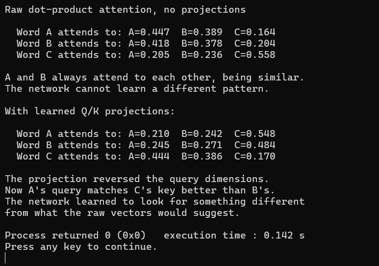
Figure 20-4 runs the same three words twice, once with the raw embeddings and once with learned projections. Without projections the geometry decides everything. Word A attends 0.447 to itself and 0.389 to B, because A and B were built to be similar, while C gets only 0.164. Word B mirrors it. Word C, being different from both, attends 0.558 to itself. There is no way to change any of this, since the scores are dot products of fixed embeddings and no parameter exists to adjust.
With the learned projections the pattern inverts. Word A now attends 0.548 to C and only 0.242 to B, so the position it previously found least relevant has become the one it attends to most. C in turn attends 0.444 to A. The embeddings did not move, and the similarity between A and B is exactly what it was. What changed is that the query and key projections send them into a space where the alignment is different.
That is the freedom the chapter is arguing for. Relevance no longer has to mean similarity in embedding space, so a model can learn that determiners attend to nouns and verbs attend to subjects without those words needing similar embeddings. It can also learn the opposite of what the raw geometry suggests, which the reversal here demonstrates directly.
20.6 The Complete Attention Function
Everything now packages into one function that takes a sequence and three matrices and returns both the weight matrix and the output vectors. This is the block that Chapter 24 stacks into a transformer, so having it in a reusable form pays off later.
/* 109_Attention_Fn.c */
#include <stdio.h>
#include <math.h>

#define SL 4    /* sequence length */
#define DM 4    /* model dimension */
#define DK 3    /* query and key dimension */
#define DV 3    /* value dimension */

static void softmax(float *x, int n)
{
    float mx = x[0], s = 0;
    int i;
    for (i = 1; i < n; i++) if (x[i] > mx) mx = x[i];
    for (i = 0; i < n; i++) {
        x[i] = expf(x[i] - mx);
        s += x[i];
    }
    for (i = 0; i < n; i++) x[i] /= s;
}

/* Q/K/V attention over one sequence. Writes the
   weight matrix and the output vectors. */
static void attention(const float X[SL][DM],
                      const float WQ[DK][DM],
                      const float WK[DK][DM],
                      const float WV[DV][DM],
                      float W[SL][SL],
                      float out[SL][DV])
{
    float Q[SL][DK], K[SL][DK], V[SL][DV];
    int i, j, k;

    for (i = 0; i < SL; i++) {
        for (k = 0; k < DK; k++) {
            Q[i][k] = 0;
            K[i][k] = 0;
            for (j = 0; j < DM; j++) {
                Q[i][k] += WQ[k][j] * X[i][j];
                K[i][k] += WK[k][j] * X[i][j];
            }
        }
        for (k = 0; k < DV; k++) {
            V[i][k] = 0;
            for (j = 0; j < DM; j++)
                V[i][k] += WV[k][j] * X[i][j];
        }
    }

    for (i = 0; i < SL; i++) {
        for (j = 0; j < SL; j++) {
            W[i][j] = 0;
            for (k = 0; k < DK; k++)
                W[i][j] += Q[i][k] * K[j][k];
        }
        softmax(W[i], SL);

        for (k = 0; k < DV; k++) {
            out[i][k] = 0;
            for (j = 0; j < SL; j++)
                out[i][k] += W[i][j] * V[j][k];
        }
    }
}

int main(void)
{
    float X[SL][DM] = {
        {  1.0f,  0.0f,  0.5f, -0.2f },   /* the  */
        {  0.3f,  0.8f, -0.1f,  0.6f },   /* cat  */
        { -0.2f,  0.1f,  0.9f,  0.3f },   /* sat  */
        {  0.5f, -0.3f,  0.2f,  0.7f },   /* down */
    };
    const char *words[SL] = {
        "the", "cat", "sat", "down"
    };

    /* Same chosen projections as Step 2 */
    float WQ[DK][DM] = {
        { -0.54f, +0.23f, +1.14f, +0.16f },
        { +1.01f, +0.59f, +3.72f, -0.67f },
        { +1.27f, +0.30f, -1.02f, +3.80f },
    };
    float WK[DK][DM] = {
        { +0.92f, -0.40f, +0.21f, +0.11f },
        { +0.16f, +0.92f, -0.18f, +0.33f },
        { -0.26f, -0.38f, +0.83f, +0.78f },
    };
    /* W_V picks out different content from W_K, which
       is the whole point of keeping them separate */
    float WV[DV][DM] = {
        { +1.00f, +0.00f, +0.00f, +0.00f },
        { +0.00f, +1.00f, +0.00f, +0.00f },
        { +0.00f, +0.00f, +1.00f, +0.00f },
    };

    float W[SL][SL], out[SL][DV];
    int i, j;

    attention(X, WQ, WK, WV, W, out);

    printf("Attention weights, rows "
           "query, cols key\n\n");
    printf("          ");
    for (j = 0; j < SL; j++) printf("%-6s", words[j]);
    printf("\n");
    for (i = 0; i < SL; i++) {
        printf("  %-6s  ", words[i]);
        for (j = 0; j < SL; j++)
            printf("%.3f ", W[i][j]);
        printf("\n");
    }

    printf("\nOutput vectors, d_v=%d\n\n", DV);
    for (i = 0; i < SL; i++)
        printf("  %-6s  [%+.3f, %+.3f, %+.3f]\n",
               words[i], out[i][0],
                   out[i][1], out[i][2]);

    printf("\nEvery row of the weight matrix sums to "
           "1.\n");
    printf("Parameters: W_Q %dx%d + W_K %dx%d + W_V "
           "%dx%d"
           " = %d\n", DK, DM, DK, DM, DV, DM,
           (DK + DK + DV) * DM);

    return 0;
}
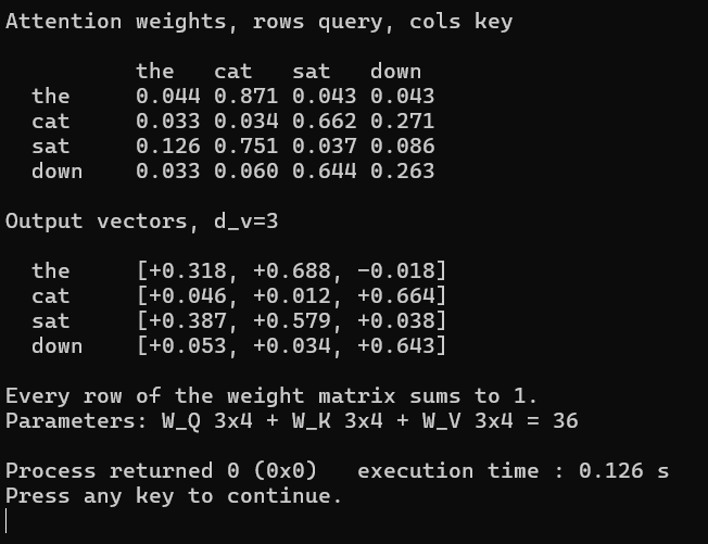
Figure 20-5 has the full weight matrix and the vectors it produces. The weight matrix is the object people mean when they show an attention map. It is square, with one row per query position and one column per key position, and every row sums to 1 because each row is a separate softmax. Reading down a column tells you how much attention a position receives, and reading across a row tells you where it looks.
The output vectors underneath are what actually leaves the layer, and they now differ per position, which is what a working attention layer should produce. Look at the row for “the”, which comes out as [+0.318, +0.688, −0.018]. W_V here is the identity on the first three components, so the value vector for “cat” is simply [0.3, 0.8, −0.1], and since “the” put 0.871 of its weight on “cat” the output is very nearly cat’s value with a small contribution from the rest. Multiply it out and 0.871 times 0.8 is 0.697, which lands within a hundredth of the 0.688 printed.
Compare that against “cat” itself, whose output is [+0.046, +0.012, +0.664] and looks nothing like it. “cat” attends mostly to “sat”, whose value is [−0.2, 0.1, 0.9], and the third component dominating the output is exactly what you would expect from that. Two adjacent positions, two completely different outputs, both computed from the same three matrices.
The parameter count printed at the end is worth registering. Three matrices of 3 by 4 gives 36 weights for this toy, and the general form is (2 * d_k + d_v) * d_model. At the transformer scale of Chapter 24, with d_model of 512 and d_k and d_v of 64, that is 98,304 per attention head.
20.7 Self-Attention and Cross-Attention
The function just built serves both patterns without modification, and the only difference is where the three inputs come from.
Self-attention draws Q, K and V from the same sequence, so every position attends to every position of the input it belongs to, including itself. That is what we ran over the sequence earlier and what a transformer uses inside its encoder layers and inside its decoder layers.
Cross-attention draws Q from one sequence and K and V from another. In an encoder-decoder transformer the decoder supplies the queries and the encoder supplies the keys and values, which is the seq2seq attention of Chapter 19 rewritten with projections in front of it. The weight matrix is no longer square in this case, since a decoder of three positions attending over an encoder of five produces a 3 by 5 matrix, and exercise 3 asks you to build exactly that.
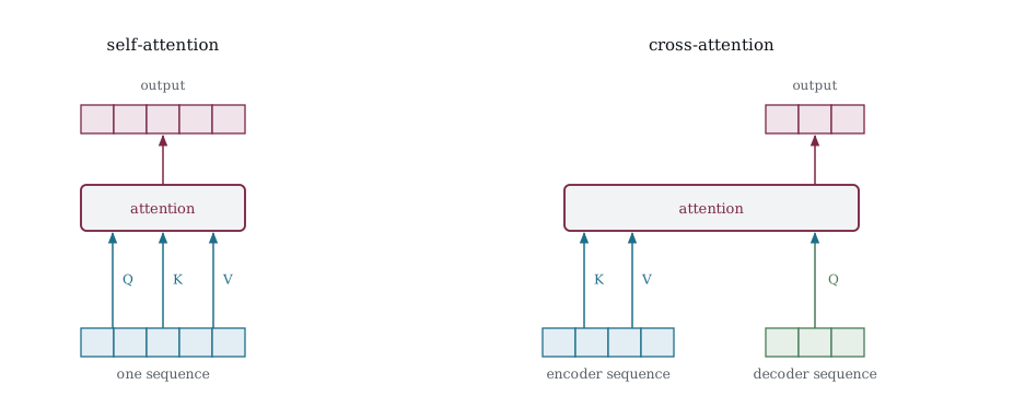
Figure 20-6 puts the two side by side. The attention block is the same block in both panels, and the only thing that differs is which sequence each of the three arrows starts from. On the left all three leave the same row. On the right the keys and values leave the encoder and the query leaves the decoder, which is also why the output has the decoder’s length rather than the encoder’s.
Nothing else changes. The same code path, the same formula and the same three matrices in the same three slots.
20.8 Key Takeaways
Three learned matrices project each input into a query, a key and a value, which separates what a position searches for from what it can be matched on from what it contributes.
We put one input of [0.5, −0.2, 0.8, 0.1] through the three matrices and got a query of [+0.510, −0.180, −0.120] and a key of [−0.030, +0.250, +0.470], disagreeing in sign on two of three components. Projections that produced similar vectors would be wasting two of the three matrices.
Without projections, attention is locked to the geometry of the embeddings. We measured word A attending 0.389 to a similar word B and 0.164 to a dissimilar C, with no parameter available to change it.
With projections the same three words reversed, A attending 0.548 to C and 0.242 to B. Relevance stopped meaning similarity in embedding space, which is the freedom the projections buy.
W_Q, W_K and W_V are shared across all positions. One set of matrices produced four different attention rows, differing only because the inputs differed, exactly as the shared recurrent weights worked in Chapter 13.
Every row of the attention weight matrix is a probability distribution over positions. The matrix is square for self-attention and rectangular for cross-attention, and it is what people display as an attention map.
Output vectors differ per position because the weights differ. The complete function produced [+0.318, +0.688, −0.018] for one position and [+0.046, +0.012, +0.664] for the next, since one attended to “cat” and the other to “sat”.
The complete formula is Attention(Q, K, V) = softmax(Q * K^T / sqrt(d_k)) * V, with Q = X * W_Q, K = X * W_K and V = X * W_V.
Parameters come to (2 * d_k + d_v) * d_model. With d_model of 512 and d_k and d_v of 64 that is 98,304 per head, and d_k is typically d_model divided by the head count for reasons Chapter 21 explains.
Self-attention takes Q, K and V from one sequence. Cross-attention takes Q from one and K and V from another. Same function and same formula, different inputs.
20.9 Exercises
Set W_Q = W_K = W_V = identity matrix and run 109_Attention_Fn.c. Verify it produces the same result as raw dot-product attention from Chapter 19.
What happens if d_k is very small (e.g., 1)? Each query and key is a single number. How does this limit the attention patterns the network can learn?
Implement cross-attention, where the query comes from a 3-position decoder sequence, and the keys/values come from a 5-position encoder sequence. The attention weight matrix should be [3 x 5].
Count the total parameters in Q/K/V attention with d_model = 512, d_k = d_v = 64. Compare to a fully connected layer with the same input and output size.
Compute the backward pass for W_Q. The gradient flows through the softmax, through the dot product, and into the projection. Write the chain rule for d_loss/d_W_Q.
In the attention weight matrix from 109_Attention_Fn.c, are there any positions that attend mostly to themselves? This self-attention pattern is common for “content words” that carry their own meaning.