Scaling Laws
How model size, data, and compute determine performance
32.1 What You Will Learn
Every architectural decision in the last ten chapters was justified by an argument about mechanism. Attention beats recurrence because information does not have to survive a per step multiplication, pre-norm beats post-norm because the residual path stays clean, and so on and so forth. None of that tells you how large to build the thing, how much text to train it on, or what either choice will buy. The reason is that those questions turn out to have quantitative answers, which was not obvious in advance and is the single most consequential empirical finding in the field. Kaplan and colleagues in 2020 and Hoffmann and colleagues in 2022 measured loss against model size, dataset size and compute across many orders of magnitude, and found smooth power laws rather than the plateaus and thresholds everyone expected. Loss falls as a fixed percentage for every fixed multiple of scale, with no sign of stopping inside the range anyone has tested.
The practical value of that is prediction. If performance follows a curve you can fit, then a small cheap experiment forecasts a large expensive one, and the decision to spend millions on a training run stops being a gamble. DeepSeek validated its architecture on 16 billion parameter models before committing to 671 billion, which is only sensible if the small result carries information about the large one.
This chapter works through the three relationships, then the Chinchilla result that overturned the first round of advice about how to spend a compute budget, then the formula that turns a model size and a token count into a number of floating point operations. In this chapter we’ll explore pulling apart the two claims that get conflated constantly, being the rate at which returns diminish and the amount they diminish by.
32.2 The Three Relationships
Three quantities determine how well a language model does, and performance here means loss on held-out text rather than any downstream score. N is the parameter count, D is the number of training tokens, and C is the total compute in floating-point operations. Each relates to loss by a power law with its own exponent.
A power law is worth reading carefully because the shape is easy to misunderstand or for the explanation not to be grasped rather. It says the loss is multiplied by a constant factor for each constant multiple of the input, so ten times the parameters always produces the same proportional improvement regardless of where you start. It does not say the improvement gets smaller as you scale, and the difference between those two statements is what we spend the last part of this chapter on.
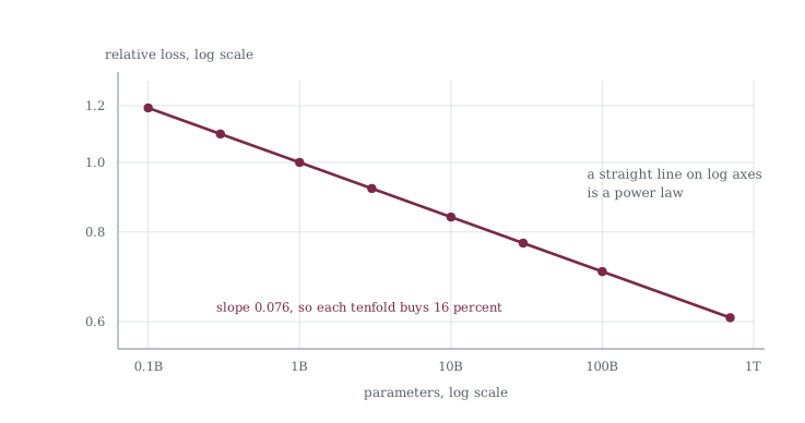
Figure 32-1 plots the first of those three laws using the numbers the program prints, on log axes for both quantities. A power law is a straight line under that treatment, and this one is straight across four orders of magnitude, from a tenth of a billion parameters to seven hundred billion. Fitting a line to those eight points recovers a slope of 0.076, which is the exponent the equation above states. Reading the same thing in percentage terms, each tenfold increase lowers the loss by about sixteen percent, and that figure staying constant is what the straightness of the line means.
The exponents are small numbers and that is the point. An exponent of 0.076 means a tenfold increase in parameters buys about sixteen percent, so the curve is shallow and the scale required to move it is enormous. That is why the field grew models by orders of magnitude rather than by percentages, and why the cost of a frontier run climbed the way it did.
/* 157_Power_Law.c */
#include <stdio.h>
#include <math.h>

int main(void)
{
    printf("Scaling laws: loss vs model size\n\n");
    printf("  %10s  %8s  %s\n", "Params",
           "Rel loss", "Improvement");
    printf("  %10s  %8s  %s\n", "----------",
           "--------", "-----------");

    /* L ~ N^(-0.076), normalized so 1B params = 1.0
       loss */
    float alpha = 0.076f;
    double sizes[] = { 1e8, 3e8, 1e9, 3e9,
                       1e10, 3e10, 1e11, 7e11 };
    int n = 8;
    double base_loss = pow(1e9, -alpha);
    int i;

    for (i = 0; i < n; i++) {
        double loss = pow(sizes[i], -alpha) / base_loss;
        printf("  %9.1fB  %8.4f  ",
               sizes[i] / 1e9, loss);
        if (i > 0) {
            double prev =
                pow(sizes[i-1], -alpha) / base_loss;
            printf("%.1f%% better",
                   (1.0 - loss/prev) * 100);
        }
        printf("\n");
    }

    printf("\n  Each 10x in parameters gives about "
           "%.0f%% lower loss.\n",
           (1.0 - pow(0.1, alpha)) * 100);
    printf("  The percentage is the same at every\n");
    printf("  scale. What shrinks is the absolute\n");
    printf("  drop, since 16%% of a smaller number\n");
    printf("  is a smaller number.\n");
    printf("  It never stops either. A bigger model\n");
    printf("  is always better, given enough data "
           "to\n");
    printf("  train it on.\n");

    return 0;
}
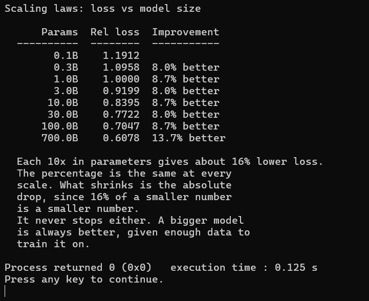
Figure 32-2 carries the same law out into a printed table. The table walks parameters from 0.1 billion to 700 billion and the relative loss falls from 1.1912 to 0.6078, normalized so a billion parameters sits at 1.0000. Each step of ten times gives sixteen percent, which the closing line states, and the alternating 8.0 and 8.7 percent figures in the improvement column are simply the alternating three times and three and a third times steps between the listed sizes rather than anything about the law.
Let’s read the whole span before moving on. Going from a hundred million parameters to seven hundred billion is a factor of seven thousand, and it takes the loss from 1.1912 to 0.6078, which is not quite a halving. Seven thousand times the model for slightly less than twice the quality is the actual exchange rate, and anyone surprised by how much frontier training costs has not looked at that number.
The last line makes a claim I want to be careful about. It says a bigger model is always better given enough data, and that holds within the range that has been measured, which spans roughly six orders of magnitude. Nobody has observed the curve bending, and nobody has shown it never will. Extrapolating a fitted power law far past the data is exactly the move that scaling law papers are careful about and popular summaries are not.
32.3 Compute Optimal Training
The 2020 result was read as saying that models should be made as large as the budget allows, with the data requirement a secondary concern, and the field spent two years acting on that reading. The 2022 Chinchilla paper showed it was wrong, and wrong in an expensive direction. For a fixed compute budget the right move is to grow model size and dataset size together rather than pouring everything into parameters, and the rule of thumb that came out of the work is roughly twenty training tokens for every parameter. Models built under the earlier advice were therefore the wrong shape and not just suboptimal, carrying parameters they had not been given enough data to make use of.
/* 158_Chinchilla.c */
#include <stdio.h>

int main(void)
{
    printf("Chinchilla optimal, about 20 tokens "
           "per parameter\n\n");

    struct {
        const char *name;
        double params;
        double tokens;
        double ratio;
    }
    models[] = {
        { "GPT-3",        175e9,   300e9,
            300e9/175e9 },
        { "Chinchilla",   70e9,    1400e9,
            1400e9/70e9 },
        { "LLaMA-7B",     7e9,     1000e9,
            1000e9/7e9 },
        { "LLaMA-70B",    70e9,    2000e9,
            2000e9/70e9 },
        { "DeepSeek-V3",  671e9,   14800e9,
            14800e9/671e9 },
    };
    int n = 5, i;

    printf("  %-12s %7s %9s %8s  %s\n", "Model",
           "Params", "Tokens", "Tok/Par", "Status");
    printf("  %-12s %7s %9s %8s  %s\n", "",
           "------", "------", "-------", "------");

    for (i = 0; i < n; i++) {
        printf("  %-12s %6.0fB %8.0fB %8.1f  %s\n",
               models[i].name,
               models[i].params / 1e9,
               models[i].tokens / 1e9,
               models[i].ratio,
               models[i].ratio < 10 ? "UNDERTRAINED" :
               models[i].ratio > 50 ? "DATA-RICH"
                                    : "BALANCED");
    }

    printf("\n  GPT-3 was undertrained at only 1.7 "
           "tokens\n  per parameter.\n");
    printf("  Chinchilla showed a 4x smaller model\n");
    printf("  on 4x more data beats it.\n\n");

    printf("  Modern models go far past that ratio.\n");
    printf("  LLaMA-7B uses 143 tokens per param,\n");
    printf("  seven times Chinchilla optimal.\n");
    printf("  DeepSeek-V3 uses 22, which is close "
           "to\n");
    printf("  optimal, but it is MoE with 37B "
           "active,\n");
    printf("  so the effective ratio is about 400\n");
    printf("  tokens per active parameter.\n");

    return 0;
}
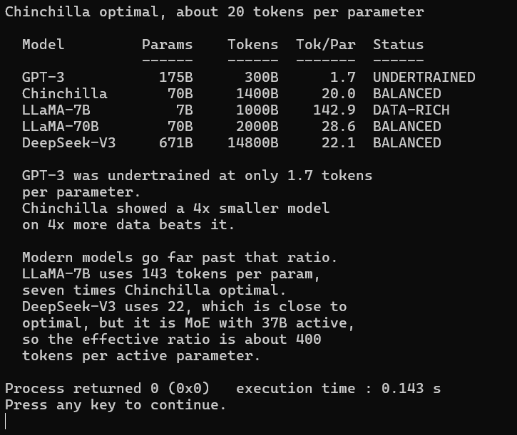
Figure 32-3 lists tokens per parameter for five real models. GPT-3 sits at the top of the table with 175 billion parameters and 300 billion tokens, which is 1.7 tokens per parameter against an optimum near 20. It was undertrained by more than a factor of ten, and Chinchilla’s own demonstration was that a model four times smaller, trained on four times more data for the same compute, beat it outright. That is a striking result, since it says the largest model of its day was the wrong shape rather than merely expensive.
The rest of the table shows what happened next, and it did not settle at twenty. LLaMA-7B uses 143 tokens per parameter, which is seven times past compute-optimal and looks wasteful by the Chinchilla criterion, though it is not a mistake. Chinchilla optimizes training compute alone, and a model that will be served to many users for a long time spends far more compute on inference than on training, so the right move is to overtrain a smaller model and pay less forever afterward. The optimum depends on which cost you are minimizing.
DeepSeek-V3′s row needs the same care in the other direction. It reads 22.1 tokens per parameter, which looks perfectly Chinchilla optimal, and the number is misleading because 671 billion is its total parameter count while only 37 billion are active for any given token. Measured against what actually runs, the ratio is closer to 400 tokens per active parameter, putting it firmly in overtrained territory alongside LLaMA rather than at the optimum. Which figure belongs in a scaling law for a mixture of experts model is a live question, and exercise 4 asks you to think it through.
32.4 The Compute Budget
Turning a model size and a token count into a cost needs exactly one formula, and after ten chapters of attention heads and residual streams it is anticlimactically simple. Every parameter is touched once per token, so the total work is the product of the two with a small constant in front.
Six floating-point operations per parameter per token. Two come from the forward pass, since a multiply-accumulate against each weight is two operations, and four come from the backward pass, which computes a gradient with respect to both the input and the weight and therefore costs roughly twice the forward. The formula ignores attention’s quadratic term, activation functions, normalization and everything else, and it is accurate to within a few tens of percent for realistic models, which is enough to plan with.
/* 159_Compute.c */
#include <stdio.h>

int main(void)
{
    printf("Training compute, C = 6 * N * D\n\n");

    struct {
        const char *name;
        /* total, what gets stored */
        double params;
        double active;      /* what runs per token */
        double tokens;
        double gpu_hours;
        double cost_per_hour;
    }
    models[] = {
        { "GPT-2 Small", 124e6, 124e6, 100e9,
          120, 2.0 },
        { "LLaMA-7B",    7e9,   7e9,   1000e9,
          82000, 2.0 },
        { "LLaMA-70B",   70e9,  70e9,  2000e9,
          1720000, 2.0 },
        /* MoE, so only 37B of the 671B run per token
           and only those cost anything to train */
        { "DeepSeek-V3", 671e9, 37e9,  14800e9,
          2788000, 2.0 },
    };
    int n = 4, i;

    printf("  %-12s %6s %6s %7s %9s %8s %6s\n",
           "Model", "Total", "Active", "Tokens",
           "FLOPs", "GPU-hrs", "Cost");
    printf("  %-12s %6s %6s %7s %9s %8s %6s\n", "",
           "-----", "------", "------", "-----",
           "-------", "----");

    for (i = 0; i < n; i++) {
        double flops =
            6.0 * models[i].active * models[i].tokens;
        double pflops = flops / 1e15;

        printf("  %-12s %5.1fB %5.1fB %6.0fB %9.1e ",
               models[i].name,
               models[i].params / 1e9,
               models[i].active / 1e9,
               models[i].tokens / 1e9,
               pflops);

        double cost = models[i].gpu_hours
                      * models[i].cost_per_hour;
        if (models[i].gpu_hours >= 1000)
            printf("%7.0fK $%5.1fM",
                   models[i].gpu_hours
                       / 1000, cost / 1e6);
        else
            printf("%8.0f $%5.1fK",
                   models[i].gpu_hours, cost / 1e3);
        printf("\n");
    }

    printf("\n  The FLOPs column uses active "
           "params,\n");
    printf("  not total. A dense model has one "
           "number\n");
    printf("  for both, and an MoE does not, since "
           "a\n");
    printf("  token only touches the experts it is\n");
    printf("  routed to. Using 671B here would give\n");
    printf("  6.0e10 PF, which against 2788K "
           "GPU-hours\n");
    printf("  works out at 5.9 PFLOP/s per GPU, "
           "well\n");
    printf("  past what the hardware can reach.\n\n");

    printf("  DeepSeek-V3: $5.6M total training "
           "cost.\n");
    printf("  GPT-4 is estimated at $100M or more.\n");
    printf("  The gap comes from architecture, "
           "since\n");
    printf("  MoE activates 37B of 671B, and from\n");
    printf("  engineering, FP8 and DualPipe.\n");

    return 0;
}
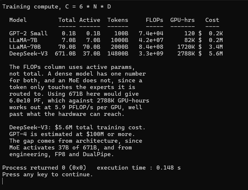
Figure 32-4 applies the compute formula, taking active parameters for the MoE. The table runs that formula across four models and the span is the first thing I want you to notice. GPT-2 Small comes to 7.4e4 petaflops and a couple of hundred dollars of compute, while DeepSeek-V3 comes to 3.3e9 petaflops and 5.6 million, which is five orders of magnitude apart in cost for models separated by about four orders of magnitude in size and two in data.
The column that needed correcting is the parameter count used in the formula. For a dense model the total and the active count are the same number, and for a mixture of experts they are not, because a token is routed to a few experts and never touches the rest. Training cost follows what runs rather than what is stored, so the formula takes the 37 billion active parameters rather than the 671 billion total.
That distinction is checkable rather than a matter of taste, and the listing does the check. Using the total would give 6.0e10 petaflops, and dividing that by the published 2,788,000 GPU-hours implies each GPU sustained 5.9 petaflops per second. An H800 peaks around one petaflop per second in its fastest format, so the total-parameter figure demands roughly six times what the hardware can physically do. The active-parameter figure gives 3.3e14 operations per second per GPU, which is a plausible fraction of peak and consistent with a real training run.
The cost comparison at the bottom is the reason the chapter mentions DeepSeek at all. Reaching frontier performance for 5.6 million dollars against an estimated hundred million or more for GPT-4 is not a scaling law result, it is an efficiency result, and efficiency multiplies the effective budget. Mixture of experts reduces the active parameter count, low precision training reduces the cost per operation, and better pipelining reduces the time GPUs spend idle. None of that changes the curve, it changes how far along the curve a given amount of money reaches.
32.5 What Diminishing Returns Actually Means
Two claims get run together whenever anyone discusses scaling, and only one of them is true. The first is that each tenfold increase in compute buys a smaller percentage improvement than the tenfold before it. The second is that each tenfold increase buys a smaller absolute reduction in loss. Both sound like the same statement in casual conversation and they are not, since one describes a rate that changes and the other describes a fixed rate applied to a shrinking quantity. This program prints both columns side by side so there is no room to confuse them.
/* 160_Emergence.c */
#include <stdio.h>
#include <math.h>

int main(void)
{
    /* L ~ C^(-0.05), so a factor of ten in compute
       multiplies the loss by 10^(-0.05) every time,
       whatever the compute already was. */
    double compute = 1;
    int i;

    printf("Loss against compute, L ~ C^-0.05\n\n");
    printf("  compute       rel loss     drop   "
           "absolute\n");
    printf("  step          at start   per 10x   "
           "    drop\n");
    printf("  -----------   --------   -------   "
           "--------\n");

    for (i = 0; i < 6; i++) {
        double loss = pow(compute, -0.05);
        double next = pow(compute * 10, -0.05);
        double pct = (1.0 - next / loss) * 100;
        printf("  %.0e -> %.0e  %8.4f  %6.1f%%  "
               "%7.4f\n",
               compute, compute * 10, loss, pct,
               loss - next);
        compute *= 10;
    }

    printf("\n  The percentage never moves. Every\n");
    printf("  factor of ten buys the same 10.9%%, "
           "which\n");
    printf("  is what a power law means.\n\n");

    printf("  The absolute column tells the other "
           "half\n");
    printf("  of the story. Read the first and last\n");
    printf("  rows of it against each other. The "
           "same\n");
    printf("  10.9%% is worth far less by the end,\n");
    printf("  because a constant fraction of a "
           "smaller\n");
    printf("  number is less. That is where the "
           "sense\n");
    printf("  of diminishing returns comes from, "
           "and\n");
    printf("  it is about the absolute drop rather\n");
    printf("  than the rate.\n");

    return 0;
}
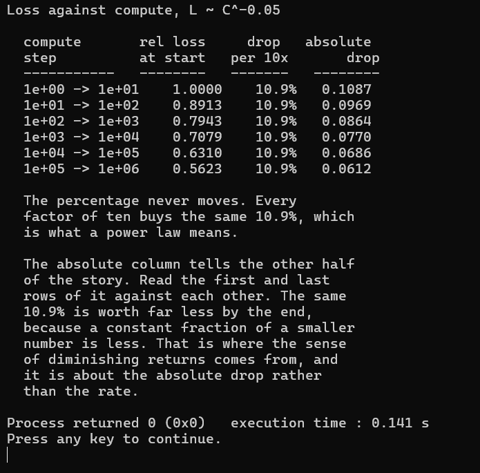
Figure 32-5 sets the rate of improvement beside the amount of it. The percentage column reads 10.9 six times in a row. It does not decay or drift, and it will read 10.9 for as many rows as anyone cares to compute, because that is what an exponent of 0.05 means. Every factor of ten multiplies the loss by 10 to the power of negative 0.05, which is 0.891, forever.
The absolute column tells the other half. The first tenfold step removes 0.1087 of loss and the sixth removes 0.0612, so the same constant percentage is worth progressively less because it is a percentage of a shrinking number. That is the real content of diminishing returns, and it is a statement about arithmetic rather than about any property of neural networks going soft at scale.
Getting this backward matters practically rather than just pedantically. If the rate were decaying then scaling would eventually stop paying and there would be a natural place to stop. It is not decaying, so there is no such place, and the decision about when to stop scaling is an economic one about whether the next order of magnitude of spending is worth 10.9 percent rather than a technical one about whether the curve has run out.
The chapter’s other topic belongs here too, since emergent abilities are usually offered as evidence against smooth scaling. Chain-of-thought reasoning, in-context learning and reliable code generation all appear to switch on somewhere rather than improving gradually, and the debate is whether that is real or an artifact. The case for artifact is strong, because a metric like exact-match accuracy has a threshold built into it, so a model whose underlying probability of a correct answer is climbing smoothly will score zero and then suddenly not. What nobody disputes is that the loss itself moves smoothly throughout, which is what these tables measure.
32.6 What the Laws Are Good For
Five consequences follow from the curves, and setting them out plainly is what makes scaling laws an engineering tool instead of a talking point. Each one is a decision somebody has to make with money attached.
Prediction is the first and the most valuable. A model trained at one percent of the budget lands on the same curve as the full run, so a small experiment forecasts a large one, and the forecast is quantitative rather than directional. DeepSeek validated its architecture on 16 billion parameter models before committing to 671 billion, which turns an enormous bet into a calculation.
Allocation is the second. For a fixed compute budget, Chinchilla says how to split it between model size and data, and we saw earlier that the answer moves once inference cost enters the picture. Training compute alone points at twenty tokens per parameter, and a model that will serve requests for years points at considerably more.
Architecture search is the third and it depends on an assumption I want to name. If a change improves loss at small scale it usually improves loss at large scale, so architectures can be compared cheaply. That assumption mostly holds and is not guaranteed, and the interesting failures in the literature are changes that helped at one scale and did nothing at another.
Then the two that pull against each other. Diminishing returns in the absolute sense means the gap between 7 billion and 70 billion parameters is worth far more than the gap between 70 billion and 700 billion, so at some point better data, better post-training and better architecture beat more scale. And efficiency multiplies whatever budget exists, which is how DeepSeek-V3 reached performance comparable to much more expensive models at roughly a twentieth of the estimated cost.
32.7 Key Takeaways
Loss follows smooth power laws in parameters, data and compute, with exponents of about 0.076, 0.095 and 0.050, validated across many orders of magnitude.
A power law means a constant proportional improvement per constant multiple of scale. It does not mean the rate of improvement decays, and conflating those two is the commonest error in discussions of scaling.
We measured a fall from 1.1912 to 0.6078 across a factor of seven thousand in parameters, which is not quite a halving of loss. That exchange rate is why frontier training costs what it does.
The Chinchilla rule is about twenty tokens per parameter for compute-optimal training. GPT-3 ran at 1.7, undertrained by more than a factor of ten, and a model four times smaller on four times more data beat it at equal compute.
Modern models deliberately overtrain, with LLaMA-7B at 143 tokens per parameter. Chinchilla optimizes training compute alone, and a model that will be served for years should minimize inference cost instead.
Compute is about 6 * N * D, being two operations per parameter per token forward and four back. It ignores everything else and is accurate enough to plan with.
For a mixture of experts the formula takes active parameters rather than total. DeepSeek-V3 uses 37 billion of 671 billion, giving 3.3e9 petaflops rather than 6.0e10.
That correction is checkable. The total-parameter figure divided by the published 2,788,000 GPU-hours implies 5.9 petaflops per second per GPU, which is around six times what an H800 can reach.
The same 671 against 37 billion distinction makes DeepSeek-V3′s 22.1 tokens per parameter closer to 400 per active parameter, which moves it from apparently optimal to firmly overtrained.
The last table printed 10.9 percent six times in a row while the absolute drop fell from 0.1087 to 0.0612. The rate is constant and the amount shrinks, which is the whole of diminishing returns.
Because the rate does not decay, there is no scale at which the curve naturally stops paying. When to stop is an economic question about whether the next order of magnitude is worth 10.9 percent.
Efficiency multiplies the effective budget without touching the curve. DeepSeek-V3 reached comparable performance at 5.6 million dollars through mixture of experts, low precision training and better pipelining.
32.8 Exercises
Using the power law L N^(-0.076), compute how many parameters you need to halve the loss relative to a 1B parameter model.
A company has a budget for 1e21 FLOPs. Using C = 6*N*D and the Chinchilla ratio D = 20*N, what is the optimal model size? How many tokens?
Plot (or print) the scaling curve for three models, fixed N with increasing D, fixed D with increasing N, and fixed C with optimal N/D split. Which curve is steepest?
DeepSeek-V3 uses MoE with 671B total but 37B active parameters. For scaling law purposes, is N = 671B or 37B? The paper shows it performs like a dense model between these sizes.
If training a 7B model costs $100K and a 70B model costs $10M, what is the cost scaling exponent? (As a hint, cost N^alpha * D, and D scales with N for Chinchilla.)
At what point do scaling laws suggest diminishing returns make it better to invest in data quality, post-training (RLHF), or architecture innovation rather than raw scale?