The Perceptron
A single neuron, weights, bias, and activation
1.1 What You Will Learn
We start at the very beginning, with the base unit of computation in every modern intelligent system. By the end of this chapter you will have built a single artificial neuron from scratch in C, and although the exercise looks trivial I would ask you to do it anyway, because every concept that follows assumes you already understand the artificial neuron we call the perceptron. You will see what weights, bias and activation functions actually do, and you will watch your neuron learn to solve a problem by adjusting its own parameters. We build everything in small steps, adding to what came before rather than replacing it. I will not drown you in mathematical formulas, and wherever a mathematical idea is needed I will explain it immediately before it gets used so that you meet the application at the same time as the notation. Mathematics turns out to be far more accessible than most people expect once the application is sitting in front of you. A theme of this book is that every step compiles on its own, so you can run each program self contained without worrying about packages or versions, and all you need is a C compiler.
1.2 The Idea
A biological neuron is one of the smallest parts of our nervous system, an electrically excitable cell that receives signals from other neurons, and together these cells form the networks that carry out everything the brain does. The mechanism deserves one sentence before we leave the biology behind, which is that a neuron sums the signals arriving at it and fires when the combined signal is strong enough. We will not deliberate on it any further than that, but you should know where the idea of the perceptron came from.
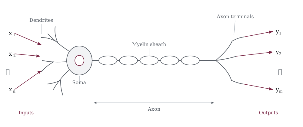
Figure 1-1 is the cell the whole idea was copied from. In the 1940s McCulloch and Pitts published the paper that introduced the idea of an artificial neuron and the artificial neural network built out of them, and in the 1950s a psychologist named Frank Rosenblatt turned that idea into mathematics and called the result the perceptron. The perceptron as we will come to know it looks like this.
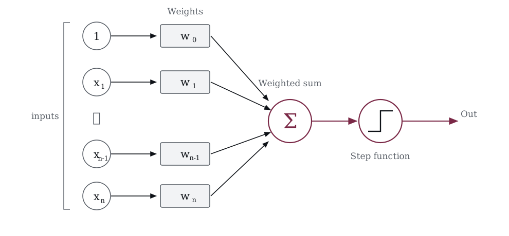
Figure 1-2 is the artificial version. The idea is simple enough that it almost sounds like a letdown when you break it down, because all a perceptron does is take numbers in, multiply each one by a weight, add everything up, and decide whether to output a 1 or a 0. That really is the entire idea, and every neural network ever built, from the simplest classifier to the largest language model in production today, is made of variations on this one unit.
Let us build one.
1.3 The Weighted Sum
We will build the perceptron by starting with the most basic version we can write and then adding features and refining it until we have a complete unit capable of real work. The most basic thing a neuron does is combine its inputs, and each input gets multiplied by a weight, which is a number controlling how much that input matters, so a large weight means the input has a strong influence on the output while a small weight means it barely contributes at all.
Suppose you have two inputs x1 and x2, where the simplest possible combination is just to add them.
But that treats both inputs equally. Weights let the neuron decide how much to care about each one. With weights w1 and w2, the weighted sum becomes.
We call this result z, and the choice of letter is a convention borrowed from linear algebra and statistics, where z denotes a linear combination of inputs before any transformation has been applied to it. If you have done algebra before then you used x for the input and y for the output, and z sits between the two as the weighted sum on its way to whatever eventually produces the final output y. That weighted sum is called a dot product, which means we multiply pairwise and then sum.
Right now w1 pairs with x1 and w2 pairs with x2, so we multiply each pair and add the two products together, and simple as the operation is; it remains the core computation of every neural network. What I also need you to understand is that nothing stops us from adding w3 with x3 and w4 with x4 and continuing as far as we care to go, and a neural network is in large part a great many of these dot products running in parallel.
If you have a background in systems programming and worked with digital signal processors before then you already understand the gist of the dot product as you may have met something called a MAC, short for multiply accumulate. What a MAC does is it computes a = a + (b * c) in a single instruction and is exactly one step of a dot product. DSPs handle that in one cycle, and neural network accelerators such as NPUs, TPUs and GPU tensor cores are essentially massive arrays of MACs, which is why we describe them as vector processing units. Vector processing performs the same operation on many data elements simultaneously and it is common to have some sort of vector processing unit in “AI” capable silicon that perform these operations.
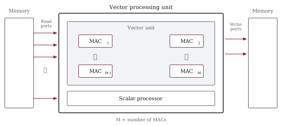
Figure 1-3 builds a vector processing unit out of an array of those MACs. Before we stray too much, let’s get back to focusing on building our perceptron. Now that you have a good understanding of how the weighted sum works, let us express it in C.
/* 000_Weighted_Sum.c */
#include <stdio.h>

int main(void)
{
    float x1 = 1.0f, x2 = 0.0f; /* inputs */
    float w1 = 0.5f, w2 = 0.5f; /* weights */

    float z = w1 * x1 + w2 * x2;

    printf("z = %.2f\n", z);

    return 0;
}

The output is in Figure 1-4. That is a rather simple program, two multiplies and an add, and the best way to understand how the weighted output behaves is to play with it. Change the inputs and the weights and run it again to build an intuition for how z responds, and you will find that when both inputs are 1 and both weights are 0.5 the result is 1.0, while when both inputs are 0 the result is 0.0 no matter what the weights happen to be.
1.4 Adding the Bias
So far our perceptron does what it has to do, taking numbers at the input and giving a number at the output, but the weighted sum on its own carries a problem that stops it from being a proper perceptron, which is that z is always zero whenever every input is zero. We need a way to shift the threshold, and that is what the bias does, being an extra number added to z.
The bias lets the neuron fire, or refrain from firing, even when the inputs are all zero, and if you have a background in electronics you can think of it as the offset voltage in an op-amp circuit. You may be wondering whether we could manage without one. Without a bias the neuron is locked to zero whenever all its inputs are zero, and no combination of weights can change that because anything multiplied by zero is still zero, which leaves the neuron able to scale its inputs but never to shift them. In practice the correct decision boundary is almost never sitting at zero. If you remember the line equation y = mx + b from school then you already know what the bias does, since the constant b is exactly what moves the line away from the origin, and without it every line the neuron is capable of learning must pass through zero, which severely limits what it can represent. Now we can add our bias.
/* 001_Bias.c */
#include <stdio.h>

int main(void)
{
    float x1 = 0.0f, x2 = 0.0f; /* inputs */
    float w1 = 0.5f, w2 = 0.5f; /* weights */

    float b = -0.7f; /* bias */

    float z = w1 * x1 + w2 * x2 + b;

    printf("z = %.2f\n", z);

    return 0;
}

Figure 1-5 adds the bias. Even with zero inputs, z is −0.7 because of the bias. The bias shifts the decision point take note of this as this will matter when we train the neuron.
1.5 The Step Activation Function
We have a number z and what we need next is a decision, and the simplest decision rule available to us is the step function. The step function behaves like a box that outputs 1 whenever z is zero or positive and outputs 0 otherwise.
The equations represent how we express the step function mathematically, but since it is a function in the mathematical sense and this is a practical book, in order to understand the step function properly we will represent it as a function in C for our perceptron. So with that being said, let’s add the step function to our program.
/* 002_Activation_Function.c */
#include <stdio.h>

static float step_function(float z)
{
    return z >= 0.0f ? 1.0f : 0.0f;
}

int main(void)
{
    float x1 = 1.0f, x2 = 1.0f; /* inputs */
    float w1 = 1.0f, w2 = 1.0f; /* weights */

    float b = -1.5f; /* bias */

    float z = w1 * x1 + w2 * x2 + b;

    float y = step_function(z); /* step activation */

    printf("z = %.2f  output = %.0f\n", z, y);

    return 0;
}

Figure 1-6 puts the step activation on the end. Once the activation is in place we have a complete neuron, where input goes in, the weighted sum is computed, the bias is added, and the activation function makes a decision, and that whole sequence is what we call the forward pass. Try changing x1 to 0 and running the program again, and you will get z = −0.5 with an output of 0.
1.6 The Forward Pass
Take a minute and look at the code in 002_Activation_Function.c again.
float z  = w1 * x1 + w2 * x2 + b;
float y = step_function(z);
The most important thing about it that I want you to pay attention to, is that it is two lines. That is everything a single neuron does when it receives input, with data flowing in one direction so that inputs go in at one end and a number comes out at the other. We call this process the forward pass. The name matters because later we will also have a backward pass, where the neuron looks at its mistakes and adjusts itself accordingly, but for the moment the forward pass is the whole story. Let us write it out as a sequence so that the pattern is clear.
Multiply each input by its weight
Add the products together
Add the bias
Pass the result through the activation function
The output is the neuron’s answer
That is it. Every neural network, no matter how large it grows, runs a forward pass, with data entering at one end and flowing forward through layers of neurons until an answer comes out the other end. We happen to have one neuron, and it does the same thing, just once. However, as we progress through the book you’ll see we keep adding on this simple concept until we reach all the way to LLMs.
Let us run through two examples using the same weights and bias to make sure the forward pass makes sense.
/* 003_Forward_Pass.c */
#include <stdio.h>

static float step_function(float z)
{
    return z >= 0.0f ? 1.0f : 0.0f;
}

int main(void)
{
    float w1 = 1.0f, w2 = 1.0f;
    float b  = -1.5f;

    /* Example A: both inputs high */
    float x1 = 1.0f, x2 = 1.0f;
    float z  = w1 * x1 + w2 * x2 + b;
    float y  = step_function(z);
    printf("A: x1=%.0f x2=%.0f  z=%.2f  y=%.0f\n", x1, x2, z, y);

    /* Example B: one input low */
    x1 = 1.0f;
    x2 = 0.0f;
    z  = w1 * x1 + w2 * x2 + b;
    y  = step_function(z);
    printf("B: x1=%.0f x2=%.0f  z=%.2f  y=%.0f\n", x1, x2, z, y);

    return 0;
}

Figure 1-7 runs two different input combinations through it. Same neuron, same weights, same bias. Different inputs, different outputs. In Example A, both inputs contribute enough to push z above zero, so the neuron outputs 1. In Example B, only one input contributes, z lands at −0.5, and the neuron outputs 0. The neuron does not know what the inputs mean. It does not know if x1 is a button press or a voltage reading or a pixel value. It just multiplies, adds, and decides. The meaning comes from the weights and bias, which determine how much each input matters and where the threshold sits.
Right now we are choosing those weights and that bias by hand, and the obvious question is whether the neuron could work them out on its own. That is what training is, and we will get there shortly, but first let us clean up the code so that it is easier to work with.
1.7 Putting It in a Struct
We have loose variables for weights and bias. That gets messy fast. If you did any type of development with C, then you’ll know the convention in C is to keep related data in a struct. A perceptron is just weights, a bias, and the number of inputs. The forward pass becomes a function that takes a pointer to the struct.
/* 004_Anding.c */
#include <stdio.h>

typedef struct{
  float w[2];    /* weights (fixed at 2 inputs) */
  float b;       /* bias */
} Perceptron;

static float step_function(float z)
{
    return z >= 0.0f ? 1.0f : 0.0f;
}

static float forward(const Perceptron *p, float x0, float x1)
{
    float z = p->w[0] * x0 + p->w[1] * x1 + p->b;
    return step_function(z);

}

int main(void)
{
    Perceptron p = {.w = {1.0f, 1.0f}, .b = -1.5f};

    printf("0 and 0 = %.0f\n", forward(&p, 0, 0));
    printf("0 and 1 = %.0f\n", forward(&p, 0, 1));
    printf("1 and 0 = %.0f\n", forward(&p, 1, 0));
    printf("1 and 1 = %.0f\n", forward(&p, 1, 1));
    return 0;
}
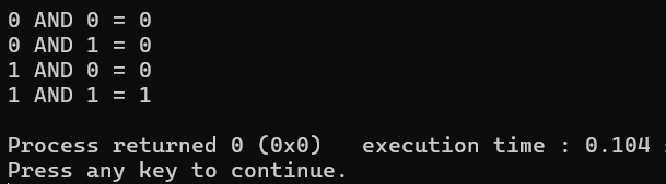
Figure 1-8 takes the struct across the whole AND truth table. We just hand picked weights (1, 1) and bias (-1.5) that make this perceptron behave like an AND gate. The forward function takes a const pointer to the struct and two inputs, computes the weighted sum plus bias, and returns the step function result. That is the same forward pass from 003_Forward_Pass.c, just organized better.
Let us verify by hand why these values work.
(0,0): z = 0 + 0 - 1.5 = −1.5 -> 0 correct
(0,1): z = 0 + 1 - 1.5 = −0.5 -> 0 correct
(1,0): z = 1 + 0 - 1.5 = −0.5 -> 0 correct
(1,1): z = 1 + 1 - 1.5 = 0.5 -> 1 correct
The weights and bias together create a dividing line in 2D space, where everything on one side outputs 1 and everything on the other outputs 0, which means the perceptron is acting as a linear classifier that draws a straight line between two categories.
1.8 Learning: The Update Rule
Up to now we have picked the weights by hand, looking at the AND truth table, thinking about it for a moment, and choosing numbers that worked. That approach is perfectly fine for two inputs and completely hopeless for a network with a thousand of them, since nobody is hand-picking a thousand weights. What we need instead is a learning algorithm that trains the perceptron for us.
Run an input through the forward pass and get the output y.
Compare y to the correct answer t (the target).
If y matches t, do nothing.
If y is wrong, nudge the weights.
I promised to keep the mathematics to a minimum and I intend to keep that promise, because the formula for training amounts to two short lines. Before we write it down it is worth restating plainly what we are trying to do, which is to have the perceptron find its own weights without us telling it what they should be. We start with bad weights, show the perceptron an example, check whether it got the right answer, and if it got the answer wrong we adjust the weights a little in the right direction, repeating that until it stops making mistakes. Here is the breakdown.
We start with zeros, setting every weight and the bias to 0.0, so that the perceptron has no opinion about anything yet.
We show it an example, picking one row from the truth table such as x0 = 1 and x1 = 0, then running the forward pass to get an output y.
We check the answer by comparing y against the target t, which is the correct answer from that row of the truth table, and subtracting one from the other to get the error.
Three things can happen from there. If the perceptron got the answer right the error is 0 and there is nothing to fix, if it should have output 1 but output 0 the error is +1, and if it should have output 0 but output 1 the error is −1. When the error is zero we move on, because the weights are already doing the right thing on this particular example, and when the error is not zero we nudge each weight by a small amount, which we can state compactly with the formula.
Sometimes it’s written as.
The i in w_i and x_i simply means whichever weight we happen to be updating, and since our perceptron carries two weights the formula runs once for w0 using input x0 and once for w1 using input x1, so writing w_i is shorthand for doing this to every weight in turn. The learning rate is written lr and is a small number we choose ahead of time, something like 0.1, which controls how large each adjustment is, and if it is too big the weights jump around wildly while if it is too small learning takes forever. The error is the +1 or −1 from above and it controls the direction, since a positive error means this weight needs to be bigger while a negative error means it needs to be smaller. The x_i is the input that this particular weight connects to, so if that input was 0 the weight did not contribute to the mistake and does not get changed, because anything times zero is zero, while if the input was 1 the weight did contribute and gets nudged accordingly.
A concrete example makes this much easier to see. Suppose w0 is currently 0.0, the input x0 is 1, the error is +1 because the perceptron should have fired and did not, and the learning rate is the 0.1 we will use in the program. The update gives us.
The weight went from 0.0 to 0.1, so the next time this input is active the weighted sum z will be a little larger and the perceptron will sit that much closer to firing, which is exactly what we wanted. The bias gets the same treatment without an input attached to it.
Which is sometimes written as.
In that case the update shifts the threshold up or down regardless of which inputs happened to be active.
One pass through all the rows of the truth table is called an epoch, and after a single epoch the weights are a little better than they were. While after several epochs the perceptron has seen every example multiple times and has gradually corrected itself. We keep going until it gets every single example right within one full epoch, meaning zero mistakes across all four rows, at which point we say the perceptron has converged and has found a set of weights that solve the problem. For the AND gate this usually takes fewer than ten epochs. If it never reaches zero mistakes we stop at a maximum number of epochs so that the program does not run forever, which will not happen for a gate as simple as AND but is good practice to have in place regardless.
Let us put that into our program. We will start all the weights at zero and let the perceptron work out AND on its own.
/* 005_Learning.c */
#include <stdio.h>

typedef struct {
    float w[2];
    float b;
} Perceptron;

static float step_function(float z)
{
    return z >= 0.0f ? 1.0f : 0.0f;
}

static float forward(const Perceptron *p, float x0, float x1)
{
    float z = p->w[0] * x0 + p->w[1] * x1 + p->b;
    return step_function(z);
}

int main(void)
{
    /* Training data: AND gate */
    float X[4][2] = { {0,0}, {0,1}, {1,0}, {1,1} };
    float T[4]    = {  0,     0,     0,     1    };

    Perceptron p = { .w = {0.0f, 0.0f}, .b = 0.0f };
    float lr = 0.1f;
    int epoch, s, i;

    for (epoch = 0; epoch < 20; epoch++) {
        int errors = 0;

        for (s = 0; s < 4; s++) {
            float y   = forward(&p, X[s][0], X[s][1]);
            float err = T[s] - y;

            if (err != 0.0f) {
                errors++;
                for (i = 0; i < 2; i++)
                    p.w[i] += lr * err * X[s][i];
                p.b += lr * err;
            }
        }

        printf("epoch %2d  errors=%d  w0=%.2f w1=%.2f b=%.2f\n",
               epoch + 1, errors, p.w[0], p.w[1], p.b);

        if (errors == 0) {
            printf("Converged!\n");
            break;
        }
    }

    /* Verify */
    printf("\nVerification:\n");
    for (s = 0; s < 4; s++)
        printf("  %.0f AND %.0f = %.0f  (expected %.0f)\n",
               X[s][0], X[s][1],
               forward(&p, X[s][0], X[s][1]), T[s]);

    return 0;
}
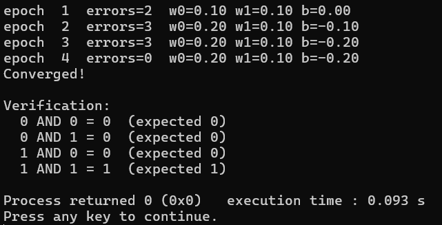
Figure 1-9 has it converging in four epochs. The weights start at zero, and on each epoch the perceptron sees all four training samples and adjusts itself in response. By epoch 4 the errors have dropped to zero and the perceptron has learned AND entirely on its own. The final weights of 0.20, 0.10 and −0.20 look nothing like the values we picked by hand, which were 1.0, 1.0 and −1.5, and yet they classify every row correctly, because there are many valid solutions to this problem and the learning algorithm found one of them.
This is the core of machine learning, where the parameters are not designed but discovered through iterative error correction. There is a convergence guarantee sitting behind it as well, which says that if the data is linearly separable, meaning a straight line can separate the two classes, then the perceptron learning algorithm is mathematically guaranteed to converge in a finite number of steps.
1.9 The Sigmoid: A Smooth Activation
So far the only activation function we have used is the step function, which works well enough for the perceptron learning rule but carries a problem that we will run straight into in Chapter 2, namely that it has no useful derivative. If you have never worked with derivatives before then the concept is a good deal simpler than the notation makes it look. Say you are driving and you check your position every second, then the derivative of your position is your speed, which tells you how fast your position is changing right now.
In a neural network we care about something very similar, since we have an error telling us how wrong the network is and we have weights that act as the knobs we can turn. The derivative of the error with respect to a weight tells us whether turning that knob a tiny amount makes the error go up or down and by how much, and that answer is exactly what lets the network work out which direction to adjust in. Remember that z is the pre-activation value, the weighted sum plus bias that we compute in the forward pass. The output of the step function is flat everywhere, giving a gradient of 0, except at the single point where z equals zero, where it jumps instantly from 0 to 1 and the gradient is infinite. You cannot do calculus on a cliff edge.
Another term thrown around a great deal is gradient, usually explained by way of partial derivatives and a long detour through notation, when the word itself simply means slope. When we say the gradient is 0 we mean the output is flat and nothing changes, so nudging z a little to the left or the right leaves the output exactly where it was, and there is no signal at all to tell the weight update which direction would be better. When the gradient is infinite then the output changes infinitely fast at a single point, which is equally useless in any real application. What we need is something in between, a smooth slope that hands us a meaningful number we can multiply by the learning rate to make a sensible update.
The function that fixes this is the sigmoid, which replaces the step function as the activation while taking the same z as its input.
Instead of a hard jump, the sigmoid produces a smooth S-shaped curve. It maps any value of z to the range (0, 1). When z is a large positive number, the output is close to 1. When z is a large negative number, the output is close to 0. When z is exactly 0, the output is 0.5. The curve is smooth everywhere, which means it has a well-defined derivative at every point. Maybe this image will clear things up a bit.
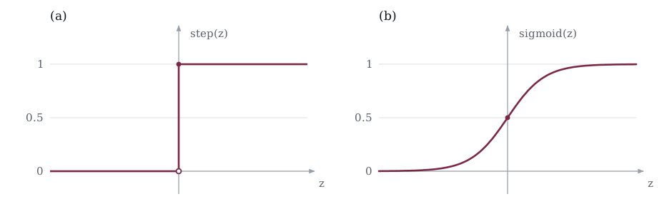
In Figure 1-10 (a) is our step function and (b) is our sigmoid function, you can see the rigidity of the step function contrasted against the smooth curves of the sigmoid. The derivative of the sigmoid has an elegant property.
Let’s break it down so you’ll understand exactly what it means. The left side, sigmoid’(z), is the gradient, which if you recall tells us how much the sigmoid output changes when we wiggle z. The right side says we can compute it using the sigmoid output we already have. If we call that output s, then the gradient is just s * (1 - s).
Let us walk through it with a number so that it makes more sense. If sigmoid(z) returned 0.8 then the gradient is 0.8 * (1 - 0.8) = 0.8 * 0.2 = 0.16, and that 0.16 tells us that nudging z by a tiny amount moves the output by about 16% of the nudge, which is a genuinely useful signal for adjusting weights. The key detail is that we never need z itself to compute the gradient, only the output we already computed during the forward pass, so if you store the output then you get the gradient for free. In Chapter 2, when we start on backpropagation, that saves us from keeping track of extra values at every layer.
Let us add the sigmoid to our perceptron and see what the trained AND gate looks like once it has a smooth activation behind it.
/* 006_Smooth_Sigmoid.c */
#include <stdio.h>
#include <math.h>

static float sigmoid(float z)
{
    return 1.0f / (1.0f + expf(-z));
}

int main(void)
{
    /* Use the weights learned from step 6 */
    float w0 = 0.2f, w1 = 0.1f, b = -0.2f;

    float X[4][2] = { {0,0}, {0,1}, {1,0}, {1,1} };
    int s;

    printf("AND gate with sigmoid activation:\n");
    for (s = 0; s < 4; s++) {
        float z = w0 * X[s][0] + w1 * X[s][1] + b;
        float y = sigmoid(z);
        printf("  %.0f, %.0f  ->  z=%6.3f  sigmoid=%.4f\n",
               X[s][0], X[s][1], z, y);
    }

    /* Show the derivative at each point */
    printf("\nSigmoid derivative at each point:\n");
    for (s = 0; s < 4; s++) {
        float z = w0 * X[s][0] + w1 * X[s][1] + b;
        float sig = sigmoid(z);
        float dsig = sig * (1.0f - sig);
        printf("  %.0f, %.0f  ->  sigmoid=%.4f  derivative=%.4f\n",
               X[s][0], X[s][1], sig, dsig);
    }

    return 0;
}
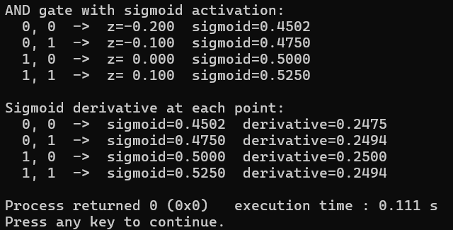
Figure 1-11 adds the derivative at each point. The outputs are no longer just 0 and 1 but soft values lying between the two, with the (0,0) case giving the lowest value and (1,1) giving the highest. If you threshold the result at 0.5 you recover exactly the same AND behavior as before, except that now you also have a gradient available at every point. The derivative column shows the gradient is largest near 0.5, where the sigmoid is at its steepest, and smallest near 0 or 1, where the curve flattens out. That gradient is what makes learning possible in deeper networks, and in Chapter 2 we will use it to train a multi-layer network with backpropagation.
1.10 What the Perceptron Cannot Do
In 1969 Minsky and Papert proved that a single perceptron cannot learn XOR. Take a look at the XOR truth table.
| x1 | x2 | x1 XOR x2 |
|---|---|---|
| 0 | 0 | 0 |
| 0 | 1 | 1 |
| 1 | 0 | 1 |
| 1 | 1 | 0 |
Seeing why takes one picture. Plot the two inputs as coordinates on a plane, so that each row of a truth table becomes a point at (x1, x2), and mark each point according to what the gate outputs there. A perceptron computes w1 * x1 + w2 * x2 + b and fires when that sum reaches zero, and the set of points where the sum is exactly zero is a straight line. Everything on one side of that line gets a 1 and everything on the other side gets a 0, which means the only question a single perceptron can ever answer is which side of a line a point falls on. Training moves the line around by adjusting the weights and the bias, but it stays a line.
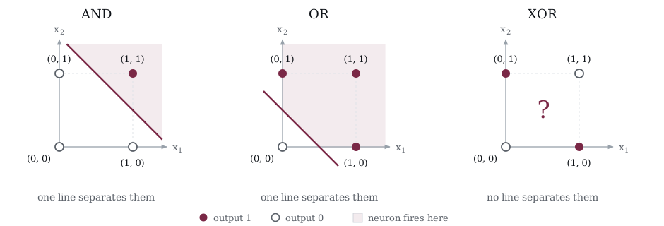
Figure 1-12 plots all three gates. For AND the single 1 sits alone in one corner, so a line tucked in across that corner does the job. For OR the single 0 sits alone in the opposite corner and the same trick works in reverse. XOR puts its two 1s on one diagonal and its two 0s on the other, and there is no way to draw a straight line with one diagonal on each side of it. The failure is geometric rather than a matter of not having trained long enough.
No single straight line can separate the 1s from the 0s when you plot these four points in 2D, because XOR is not linearly separable. Try training 005_Learning.c on XOR data by changing T to {0, 1, 1, 0} and watch it oscillate forever, since it will never converge for the straightforward reason that no solution exists for a single neuron. That result is usually credited with draining the funding and the interest out of neural network research for more than a decade. The fix is to stack neurons into layers, where a hidden layer sitting between the input and the output can learn the intermediate representations needed to solve XOR, and that is a large part of what Chapter 2 covers.
You cannot appreciate why layers matter, though, until you understand the single neuron thoroughly. You now do.
1.11 Key Takeaways
A perceptron computes z = w1 * x1 + w2 * x2 + … + wn * xn + b and passes z through an activation function, which together is the forward pass.
The step function gives a binary output of 0 or 1, while the sigmoid gives a smooth output in the range (0, 1) along with a derivative we can actually use.
The perceptron learning rule nudges each weight by lr * error * input, one pass through all the training samples is called an epoch, and the rule converges for any linearly separable problem.
A single perceptron draws a straight line, or a hyperplane in higher dimensions, to separate two classes, so it cannot solve any problem that needs a curve, XOR being the standard example.
The sigmoid derivative sigmoid(z) * (1 - sigmoid(z)) can be computed from the output alone, which is the key to backpropagation in Chapter 2.
1.12 Exercises
Modify 005_Learning.c to learn OR (target: {0, 1, 1, 1}). How many epochs to converge? Compare the learned weights to AND.
Train on NAND (target: {1, 1, 1, 0}). What happens to the sign of the bias?
Train on XOR (target: {0, 1, 1, 0}). Let it run for 1000 epochs. Confirm it never converges.
Extend the perceptron to 3 inputs and train on a 3-input AND gate. What changes in the struct and the forward function?
Write a function that computes the sigmoid derivative and verify it matches sig * (1 - sig) by comparing to a numerical approximation: (sigmoid(z + h) - sigmoid(z - h)) / (2 * h) with h = 0.0001.
Print the decision boundary for the trained AND gate: the line w0x0 + w1x1 + b = 0. Compute two points on this line (set x0 = 0, solve for x1, then set x1 = 0, solve for x0). Do they make sense geometrically?