The Multi-Layer Perceptron
Hidden layers and backpropagation
2.1 What You Will Learn
In Chapter 1 we built a single neuron and trained it, and then we found the wall it runs into, which is that one neuron cannot learn XOR. We break through that wall here by stacking neurons into layers. A layer is nothing more exotic than several neurons computing at the same time on the same inputs, each with its own weights and its own bias, so that where one neuron produced a single number a layer of two produces two. Nothing about the individual neuron changes. What changes is what we do with the numbers that come out of it.
The arrangement that matters is putting one layer in front of another, so that the outputs of the first become the inputs of the second. The first layer is called hidden, because its outputs are never the answer we read off. They are intermediate values that exist only to be consumed by the layer after it, and the network is free to make them whatever it finds useful. That freedom is the whole point. A single neuron has to work with the inputs it was handed, while a network with a hidden layer gets to reshape those inputs first and then decide.
Everything in the chapter follows from that one arrangement. The hidden neurons are ordinary perceptrons of the kind we already built, each computing a weighted sum and passing it through sigmoid, and the output neuron is another one that happens to read its inputs from them rather than from the world. No new component gets invented anywhere in this chapter. What we have to work out instead is how to train a neuron whose inputs are themselves being learned, because the perceptron rule from Chapter 1 knows what the correct answer at the output should be and has nothing to say about what the correct answer at a hidden neuron would even mean.
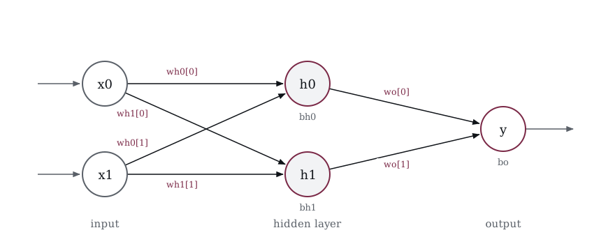
The network in Figure 2-1 is the one we build in this chapter, two inputs feeding two hidden neurons feeding one output, and it is worth reading the labels now because they are the names the code uses later. Two inputs arrive at two hidden neurons, each hidden neuron owns a weight for every input, and the output neuron owns one weight for each hidden neuron. Counting them gives four hidden weights, two hidden biases, two output weights and one output bias, so nine numbers in total. By the end of the chapter every one of those nine will have been found by the network rather than chosen by us.
You will build this two layer network from scratch, see why a hidden layer solves what a single neuron cannot, and implement backpropagation, the algorithm that makes the whole thing trainable. We build it one piece at a time.
2.2 The Problem
Here is the XOR truth table again.
| x1 | x2 | x1 XOR x2 |
|---|---|---|
| 0 | 0 | 0 |
| 0 | 1 | 1 |
| 1 | 0 | 1 |
| 1 | 1 | 0 |
If you can recall from the last chapter, the reason a single perceptron cannot learn XOR is that it draws one straight line to separate classes. In order to learn how to XOR though we need at least two lines and in order to get this done, the solution is to use multiple neurons. Some neurons draw the lines, and another neuron combines their outputs to make the final decision. The neurons that draw the lines live in a hidden layer, hidden because their outputs are not the final answer, they are intermediate computations that feed into the output neuron.
2.3 Two Neurons, Two Lines
Let us start with the smallest hidden layer worth having, which is two neurons. Each one computes a weighted sum, adds a bias, and passes the result through sigmoid. Their outputs feed into an output neuron that makes the final decision.
First, let us just get two neurons computing in sequence. No training yet. We will hand-pick weights that solve XOR so you can see the architecture work before we automate it.
/* 007_Two_Neurons.c */
#include <stdio.h>
#include <math.h>

static float sigmoid(float z)
{
    return 1.0f / (1.0f + expf(-z));
}

int main(void)
{
    /* Hidden neuron 0: learns "x0 OR x1"*/
    float wh0[2] = {20.0f, 20.0f};
    float bh0    = -10.0f;

    /* Hidden neuron 1: learns "x0 and x1" */
    float wh1[2] = {20.0f, 20.0f};
    float bh1    = -30.0f;

    float X[4][2] = { {0, 0}, {0, 1}, {1,0}, {1, 1}};
    int s;

    printf("Hidden neuron outputs:\n");

    for (s = 0; s < 4; s++)
    {
        float z0 = wh0[0]*X[s][0] + wh0[1]*X[s][1] + bh0;
        float h0 = sigmoid(z0);

        float z1 = wh1[0]*X[s][0] + wh1[1]*X[s][1] + bh1;
        float h1 = sigmoid(z1);

        printf(" x=(%.0f, %.0f)"
               " h0=%.4f h1=%.4f\n",
               X[s][0], X[s][1],
               h0, h1);
    }

    return 0;
}
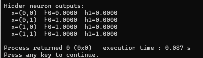
So, if we look at Figure 2-2 we see neuron h0 outputs 1 when either input is 1 (OR) and neuron h1 outputs 1 only when both inputs are 1 (AND). If we look at the h0 and h1 columns together, the XOR pattern is “h0 is on AND h1 is off” and a single output neuron can learn that. The large weights (20) make the sigmoid act almost like a step function. We are using extreme values to make the logic obvious. In practice, training will find smaller, subtler weights.
2.4 Adding the Output Neuron
Now that we understand how the internal layers work, we can look at how the output layer uses what they produce to solve the XOR problem. We add a third neuron that takes h0 and h1 as inputs and produces the final output. This output neuron needs to fire when h0 is high and h1 is low which means a positive weight for h0 and a negative weight for h1.
/* 008_Two_Neurons.c */
#include <stdio.h>
#include <math.h>

static float sigmoid(float z)
{
    return 1.0f / (1.0f + expf(-z));
}

int main(void)
{
    /* Hidden layer weights */
    float wh0[2] = {20.0f, 20.0f}; float bh0 = -10.0f;
    float wh1[2] = {20.0f, 20.0f}; float bh1 = -30.0f;

    /* Output neuron: fires when h0 is on, h1 is off */
    float wo[2] = {20.0f, -20.0f};
    float bo    =  -10.0f;

    float X[4][2] = { {0,0}, {0,1}, {1,0}, {1,1}};
    float T[4]    = {  0,     1,     1,     0   };
    int s;

    printf("Full network XOR:\n");


    for (s = 0; s < 4; s++)
    {
        /* Forward pass: hidden layer */
        float h0 = sigmoid(wh0[0]*X[s][0]
                          + wh0[1]*X[s][1] + bh0);
        float h1 = sigmoid(wh1[0]*X[s][0]
                          + wh1[1]*X[s][1] + bh1);

        /* Forward pass: output layer */
        float y = sigmoid(wo[0]*h0 + wo[1]*h1 + bo);

        printf(" x=(%.0f, %.0f) h0=%.4f"
               " h1=%.4f y=%.4f t=%.0f\n",
               X[s][0], X[s][1],
               h0, h1, y, T[s]);
    }

    return 0;
}
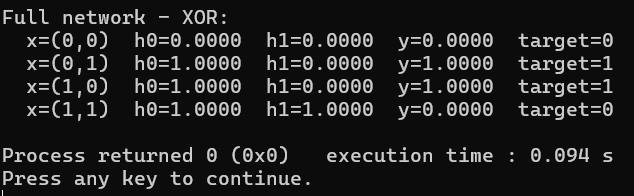
There we go, Figure 2-3 has XOR solved. The network we built to solve the problem has two layers, a hidden layer with two neurons and an output layer with one neuron. Data flows forward through both layers, this is the forward pass for a multi-layer network. The key insight I want you to take from this is that the hidden layer transforms the inputs into a new representation where XOR becomes linearly separable. The output neuron then draws a single line in that transformed space.
2.5 The Forward Pass as Arrays
We solved the XOR problem, but we cheated. We hand-picked weights that we already knew would work, just to prove the two-layer architecture can represent XOR. If we set the bias too far positive or made certain weights too small, the outputs would be wrong. The network did not learn anything; we told it the answers. Before we can train this network to find the right weights on its own, we need to organize the forward pass so it works with arrays of weights and a proper struct. This is the same cleanup we did in Chapter 1, but now for two layers.
/* 009_Pass_as_Arrays.c */
#include <stdio.h>
#include <math.h>

static float sigmoid(float z)
{
    return 1.0f / (1.0f + expf(-z));
}

/* 2 input, 2 hidden, 1 output network */
typedef struct {
    float wh[2][2];   /* wh[neuron][input] */
    float bh[2];
    float wo[2];      /* output weights, one per hidden */
    float bo;
} Net;

/* Forward pass. Stores hidden outputs in h[]. */
static float forward(const Net *n,
                     const float x[2], float h[2])
{
    int i, j;

    /* Hidden layer */
    for (i = 0; i < 2; i++) {
        float z = n->bh[i];
        for (j = 0; j < 2; j++)
            z += n->wh[i][j] * x[j];
        h[i] = sigmoid(z);
    }

    /* Output layer */
    {
        float z = n->bo;
        for (i = 0; i < 2; i++)
            z += n->wo[i] * h[i];
        return sigmoid(z);
    }
}

int main(void)
{
    Net net = {
        .wh = {{ 20, 20}, { 20, 20}},
        .bh = {-10, -30},
        .wo = { 20, -20},
        .bo = -10
    };

    float X[4][2] = { {0,0}, {0,1}, {1,0}, {1,1} };
    float T[4]    = {  0,     1,     1,     0    };
    float h[2];
    int s;

    for (s = 0; s < 4; s++) {
        float y = forward(&net, X[s], h);
        printf("x=(%.0f,%.0f)  y=%.4f  target=%.0f\n",
               X[s][0], X[s][1], y, T[s]);
    }
    return 0;
}
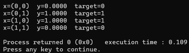
Figure 2-4 is the rewritten version. Same results, cleaner code. Notice that forward() stores the hidden layer outputs in the array h[]. We will need those values during training. When we compute gradients, we need to know what every neuron output during the forward pass.
2.6 The Loss Function
Before we can train, we need a way to measure how wrong the network is, and the way we do that is with something called a loss function. The loss function takes the network’s output y and the target t and produces a single number, and if y matches t perfectly, loss is zero. The further off y is the bigger the loss gets, and all training is doing is just pushing that number down. We can write the MSE loss function this way.
Simple, right? You should know though that in industry engineers usually write it this way instead.
This makes sense if you remember error is written as t-y. So the next obvious question is why do we square the error and there are two reasons we do this. Firstly, it makes negative errors positive. If y overshoots or undershoots, we want both to count as bad. Secondly, squaring punishes big mistakes more than small ones. Being off by 0.1 gives a loss of 0.01 but being off by 0.5 gives 0.25. The network gets penalized harder the further it drifts from the target.
Now if we have a batch of samples what we do is we average the losses. Each sample has its own error so we square each one, add them all up and divide by N, the number of samples. For XOR the value of N is 4.
The _i just means “for each sample.” Sample 0 contributes (t_0 - y_0)^2, sample 1 contributes (t_1 - y_1)^2, and so on. Dividing by N keeps the loss from growing just because you have more samples. Whether you train on 4 samples or 4000, the loss stays on the same scale.
This is all well and good but in order to know which direction we need to turn the weights we need to take the derivative of the function. The loss simply tells us how wrong the network is and not how to fix it, and telling us how to fix it is the job of the derivative. Think of it like tuning a knob, the old fashioned analog ones. The loss is the reading you see on your screen, and you want it at zero. You can’t just stare at the reading and know which way to turn, what you need to do is to nudge the pot a tiny amount, check if the reading went up or down, and that tells you the direction. The derivative is that nudge test, but computed mathematically instead of by trial and error.
That gives us the derivative of the loss with respect to y.
If y is too small (t > y), the derivative is negative, meaning we should increase y. If y is too large (t < y), the derivative is positive, meaning we should decrease y. We won’t add the derivative yet though, since I want you to understand the loss function. Let us add a loss computation to our network.
/* 010_Loss_Computation.c */
#include <stdio.h>
#include <math.h>

static float sigmoid(float z)
{
    return 1.0f / (1.0f + expf(-z));
}

typedef struct {
    float wh[2][2];
    float bh[2];
    float wo[2];
    float bo;
} Net;

static float forward(const Net *n,
                     const float x[2], float h[2])
{
    int i, j;
    for (i = 0; i < 2; i++) {
        float z = n->bh[i];
        for (j = 0; j < 2; j++)
            z += n->wh[i][j] * x[j];
        h[i] = sigmoid(z);
    }
    {
        float z = n->bo;
        for (i = 0; i < 2; i++)
            z += n->wo[i] * h[i];
        return sigmoid(z);
    }
}

int main(void)
{
    Net net = {
        .wh = {{ 20, 20}, { 20, 20}},
        .bh = {-10, -30},
        .wo = { 20, -20},
        .bo = -10
    };

    float X[4][2] = { {0,0}, {0,1}, {1,0}, {1,1} };
    float T[4]    = {  0,     1,     1,     0    };
    float h[2];
    float total_loss = 0.0f;
    int s;

    for (s = 0; s < 4; s++) {
        float y    = forward(&net, X[s], h);
        float diff = T[s] - y;
        float loss = diff * diff;
        total_loss += loss;
        printf("x=(%.0f,%.0f)  y=%.4f"
               "  target=%.0f  loss=%.6f\n",
               X[s][0], X[s][1], y, T[s], loss);
    }
    printf("Average loss: %.6f\n", total_loss / 4.0f);
    return 0;
}
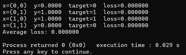
Figure 2-5 reports the loss on each sample. The loss is zero because our hand-picked weights already solve XOR perfectly. When we start training from random weights, the loss will start high and decrease as the network learns.
2.7 The Chain Rule
You now have enough knowledge to operate the network manually, what you need now is a way to train the network which is what we’ll do in this section moving forward. In Chapter 1, the perceptron learning rule was simple, we nudge each weight by the error times the input. That rule however only works for a single layer, with multiple layers, we need a way to figure out how much each weight in the hidden layer contributed to the final error. The answer is something that comes from calculus known as the chain rule. It’s a very simple concept that has been over complicated.
You know the derivative tells you which direction to nudge something to reduce the loss. But the loss depends on y, and y depends on the weights, and the weights are buried behind sigmoid functions and two layers of math. You can’t just take the derivative of the loss with respect to a hidden weight directly because there are too many steps in between.
The chain rule lets you break that big problem into small steps. Instead of asking “how does this weight affect the loss?” all at once, you ask a series of simpler questions.
How does the loss change when y changes? How does y change when the output neuron’s z changes? How does that z change when h0 changes? How does h0 change when the hidden neuron’s z changes? How does that z change when the weight changes?
Each of those is a simple derivative you can compute on its own. The chain rule then tells us to multiply them all together, and doing that gives you the answer to the original question. You usually see the chain rule formula written something like this.
This is the chain rule in two steps. You want to know, if I change weight w, how does y change? But y doesn’t depend on w directly. It depends on z, and z depends on w, this is exactly what we were discussing but in compact form, essentially what you do is break it into two questions and multiply the answers.
The term dz/dw asks how z changes when I nudge w, and since z = w*x + b, the answer is just x which is our input value.
The term dy/dz asks how y changes when z changes, and since y = sigmoid(z), this is the sigmoid derivative, which is y * (1 - y).
Multiply them together and you get dy/dw and this tells us how much the output moves for a tiny nudge to the weight. That is the amplifier gain analogy again. dz/dw is the gain of the first stage, dy/dz is the gain of the second stage, and the total gain is the product. In our network, the output y depends on the hidden outputs h, and h depends on the input weights. We need to trace the error backward through the network, layer by layer, computing how much each weight contributed to the error. This is called backpropagation.
Let us work through the math for our two-layer network before we write any code. This is the hardest part of the chapter. Take it slowly, trust me try to understand as much as you could this is the “core” of modern neural networks.
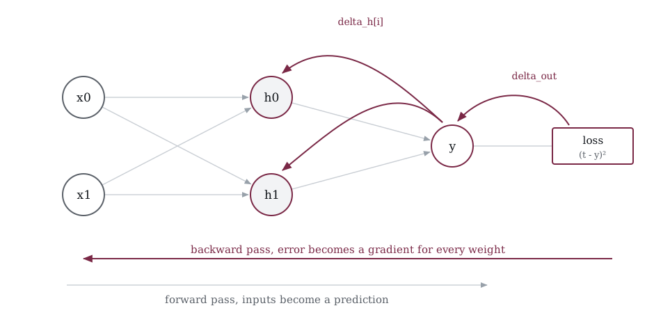
Figure 2-6 shows the shape of what we are about to derive a concept known as backpropagation. The pale arrows are the forward pass we already built, carrying inputs left to right until a number comes out. The dark arrows are the new part, carrying error right to left along those same connections. Nothing new is wired into the network for the backward pass, and the error reaches a weight by the route that weight used to influence the output. The two labeled quantities are the ones the code will compute, an output delta at y and a hidden delta at each of h0 and h1, and every weight update in the chapter is one of those deltas multiplied by whatever fed into it.
We start at the output layer.
The output neuron computes y = sigmoid(z_out) where z_out = wo[0]*h[0] + wo[1]*h[1] + bo. We want to know how each output weight affects the loss so we can fix it. The chain rule breaks this into three simple questions multiplied together.
d_loss/d_wo[i] = d_loss/dy
               * dy/dz_out
               * dz_out/d_wo[i]
The first of them asks how the loss changes when y changes, and that is the MSE derivative we just worked out, which comes to −2 * (t - y). Stepping back one link, how y changes when z_out changes is the sigmoid derivative, y * (1 - y). The last term is the easiest of the three, because z_out is nothing but a weighted sum and nudging one weight moves it by whatever that weight happens to multiply, which is h[i].
Multiplying all three gives the gradient we wanted.
d_loss/d_wo[i] = -2 * (t - y) * y * (1 - y) * h[i]For the output bias it is the same chain, except that the input for a bias is always 1.
d_loss/d_bo = -2 * (t - y) * y * (1 - y) * 1Once you understand this then you will have no problem understanding hidden layer gradients.
Now for the hidden layer.
The hidden weights are one step further from the output, so the error has to travel through an extra layer to reach them. We ask the same three questions we asked for the output weights, then tack on two more, the first being how the output neuron’s z changes when this hidden neuron’s output changes and the second being how this hidden neuron’s output changes when its own z changes. Five questions instead of three, but each one is still a simple number, and we still just multiply them all together.
To keep things tidy, we bundle the first three answers into a single number called the output delta. Think of it as the error signal sitting at the output neuron. Each hidden neuron receives that signal, scaled down by the weight connecting it to the output and by its own sigmoid derivative. That gives each hidden neuron its own delta, and from there the weight updates follow the same pattern as the output layer, which is delta times input.
We can dig into the math behind it so you’ll understand a bit better. It can get rather complicated but I will try to explain it as best I can. A hidden weight does not connect directly to the output. The error has to travel backward through the output neuron first, then through the hidden neuron. Two more questions get added to the chain.
d_loss/d_wh[i][j] = d_loss/dy
                  * dy/dz_out
                  * dz_out/dh[i]
                  * dh[i]/dz_h[i]
                  * dz_h[i]/d_wh[i][j]
The first of the new terms asks how z_out changes when h[i] changes, and the answer is the weight connecting them, wo[i]. The second asks how h[i] changes when its own z changes, and that is the sigmoid derivative again, h[i] * (1 - h[i]).
That is a lot of terms to carry around. So we bundle the first three into one number called the output delta.
delta_out = -2 * (t - y) * y * (1 - y)Think of it as “how loud is the error signal at the output neuron.” Then each hidden neuron receives that signal scaled by the weight connecting it to the output, and scaled again by its own sigmoid derivative.
delta_h[i] = delta_out * wo[i] * h[i] * (1 - h[i])Now every update is a delta multiplied by an input.
d_loss/d_wo[i]    = delta_out * h[i]
d_loss/d_bo       = delta_out
d_loss/d_wh[i][j] = delta_h[i] * x[j]
d_loss/d_bh[i]    = delta_h[i]
That is backpropagation. The error signal starts at the output and flows backward through the weights that connect the layers. Each neuron takes the upstream signal, scales it by its own sigmoid derivative, and passes it along. The weight updates at every layer follow the same pattern of learning rate times delta times input.
2.8 Backpropagation in C
Let us implement the backward pass, where we will compute the deltas, then update all weights. This is the moment everything comes together.
/* 011_Backpropagation.c */
#include <stdio.h>
#include <stdlib.h>
#include <math.h>

static float sigmoid(float z)
{
    return 1.0f / (1.0f + expf(-z));
}

typedef struct {
    float wh[2][2];   /* hidden weights [neuron][input] */
    float bh[2];      /* hidden biases */
    float wo[2];      /* output weights [hidden_neuron] */
    float bo;         /* output bias */
} Net;

static float forward(const Net *n,
                     const float x[2], float h[2])
{
    int i, j;
    for (i = 0; i < 2; i++) {
        float z = n->bh[i];
        for (j = 0; j < 2; j++)
            z += n->wh[i][j] * x[j];
        h[i] = sigmoid(z);
    }
    {
        float z = n->bo;
        for (i = 0; i < 2; i++)
            z += n->wo[i] * h[i];
        return sigmoid(z);
    }
}

static void backward(Net *n, const float x[2],
                      const float h[2],
                      float y, float t, float lr)
{
    int i, j;
    float delta_out, delta_h[2];

    /* Output delta: d_loss/dy * dy/dz_out */
    delta_out = -2.0f * (t - y) * y * (1.0f - y);

    /* Hidden deltas: error flows back through wo */
    for (i = 0; i < 2; i++)
        delta_h[i] = delta_out * n->wo[i]
                     * h[i] * (1.0f - h[i]);

    /* Update output weights and bias */
    for (i = 0; i < 2; i++)
        n->wo[i] -= lr * delta_out * h[i];
    n->bo -= lr * delta_out;

    /* Update hidden weights and biases */
    for (i = 0; i < 2; i++) {
        for (j = 0; j < 2; j++)
            n->wh[i][j] -= lr * delta_h[i] * x[j];
        n->bh[i] -= lr * delta_h[i];
    }
}

static void init_random(Net *n)
{
    int i, j;
    for (i = 0; i < 2; i++) {
        for (j = 0; j < 2; j++)
            n->wh[i][j] =
                ((float)rand() / RAND_MAX) * 2.0f - 1.0f;
        n->bh[i] = ((float)rand() / RAND_MAX) * 2.0f - 1.0f;
        n->wo[i] = ((float)rand() / RAND_MAX) * 2.0f - 1.0f;
    }
    n->bo = ((float)rand() / RAND_MAX) * 2.0f - 1.0f;
}

int main(void)
{
    float X[4][2] = { {0,0}, {0,1}, {1,0}, {1,1} };
    float T[4]    = {  0,     1,     1,     0    };
    Net net;
    float lr = 1.0f;
    int epoch, s;

    srand(42);
    init_random(&net);

    for (epoch = 0; epoch < 10000; epoch++) {
        float total_loss = 0.0f;

        for (s = 0; s < 4; s++) {
            float h[2], y, diff;

            y = forward(&net, X[s], h);
            diff = T[s] - y;
            total_loss += diff * diff;
            backward(&net, X[s], h, y, T[s], lr);
        }

        if ((epoch + 1) % 2000 == 0)
            printf("epoch %5d  loss=%.6f\n",
                   epoch + 1,
                   total_loss / 4.0f);
    }

    /* Final results */
    printf("\nFinal results:\n");
    for (s = 0; s < 4; s++) {
        float h[2];
        float y = forward(&net, X[s], h);
        printf("  %.0f XOR %.0f = %.4f  (target %.0f)\n",
               X[s][0], X[s][1], y, T[s]);
    }

    return 0;
}
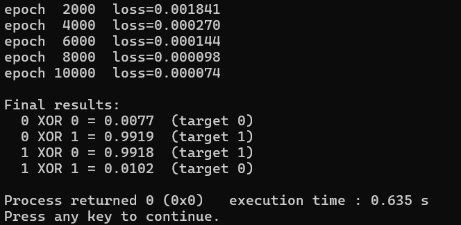
Figure 2-7 has the network learning XOR on its own. Now this was a bit much and a bit longer than the other stuff that you are accustomed to working with so far, so let’s spend some time understanding what that code is doing.
You should be familiar with much of the structure by now, so we’ll start by looking at the new function which is the backward function, and it does four things in order. First, it computes the output delta on line 42. This is the chain rule answer to “how wrong was the output and in which direction?” It multiplies the MSE derivative −2 * (t - y) by the sigmoid derivative y * (1 - y). One number that captures both how far off the prediction was and how sensitive the sigmoid is at that point. Second, it computes a delta for each hidden neuron on lines 45-46. The output delta travels backward through the output weights and each hidden neuron receives the output delta scaled by the weight connecting it to the output, then scaled again by its own sigmoid derivative h[i] * (1 - h[i]). This is the error signal arriving at the hidden layer.
Third, it updates the output weights on lines 49-51. Each weight gets nudged by learning rate times delta times the input to that weight. For the output layer, the inputs are the hidden neuron outputs h[i]. The bias update is the same but with no input to multiply, since the bias input is always 1 and lastly, it updates the hidden weights on lines 54-57. It’s the same pattern, just one layer deeper, the learning rate is times delta times input, but now the delta is the hidden delta and the input is x[j] from the original sample.
The other new function, the init_random function fills every weight and bias with a random value between −1 and 1. Unlike the previous listing where we hand-picked weights, this time the network starts knowing nothing. The srand(42) on line 81 seeds the random number generator so the results are reproducible.
The training loop on lines 84-98 is where everything comes together. For each epoch, it runs all four samples through the network. For each sample it calls forward to get a prediction, computes the loss, then calls backward to adjust the weights. After 10,000 epochs of this, the network has seen each sample 10,000 times and had 10,000 chances to correct its weights. The loss should be near zero by the end, meaning the network learned XOR on its own.
After we run it, we will see the loss decrease over thousands of epochs. The final outputs come out close to the XOR targets, near 0 for (0,0) and (1,1) and near 1 for (0,1) and (1,0). One thing to note is that the learning rate is 1.0, which is large. XOR is a small problem and can handle aggressive updates. For larger networks we will use smaller learning rates. I should also mention that the network may not converge every time with random initialization. Some starting points lead to bad local minima. Try different seeds if it gets stuck. This is a real issue in neural networks that we will address in later chapters with better initialization and optimizers.
If you have any exposure to the field before, one of the things you are sure to have heard about is something called gradient descent. The gradient if you remember is the slope and this points uphill, so what we do is we go in the opposite direction. That is why our weight updates use -= in our backward function. The gradient tells us which direction would make the loss worse, so we step the other way, and taking one small step drops the loss a little while taking another drops it again. Keep stepping and eventually you reach a low point where the network’s predictions are close to the targets. That whole business of measuring the slope, stepping downhill and repeating is gradient descent, and the learning rate controls how big each step is. Too big and you overshoot the low point, bouncing back and forth without settling. Too small and training takes forever because each step barely moves. The value 1.0 we use here is aggressive, but it works for a problem as simple as XOR. A lot of people over complicate what gradient descent is, but now you have a good idea and know exactly what it is.
2.9 Watching It Learn
Now we’re at the point where we can see the payoff for the whole chapter. We first started by handpicking weights to prove the architecture works, then we added a loss function to measure how wrong the network is.. Then we added backpropagation to fix the weights automatically, now we open the lid and verify that the network actually found a valid solution without telling up the answer. With that being said, let us add some instrumentation to see what the hidden layer learns and after training, we will print the hidden neuron outputs for each input to see what representations the network discovered.
/* 012_Watching_It_Learn.c */
#include <stdio.h>
#include <stdlib.h>
#include <math.h>

static float sigmoid(float z)
{
    return 1.0f / (1.0f + expf(-z));
}

typedef struct {
    float wh[2][2];
    float bh[2];
    float wo[2];
    float bo;
} Net;

static float forward(const Net *n,
                     const float x[2], float h[2])
{
    int i, j;
    for (i = 0; i < 2; i++) {
        float z = n->bh[i];
        for (j = 0; j < 2; j++)
            z += n->wh[i][j] * x[j];
        h[i] = sigmoid(z);
    }
    {
        float z = n->bo;
        for (i = 0; i < 2; i++)
            z += n->wo[i] * h[i];
        return sigmoid(z);
    }
}

static void backward(Net *n, const float x[2],
                      const float h[2],
                      float y, float t, float lr)
{
    int i, j;
    float delta_out, delta_h[2];

    delta_out = -2.0f * (t - y) * y * (1.0f - y);

    for (i = 0; i < 2; i++)
        delta_h[i] = delta_out * n->wo[i]
                     * h[i] * (1.0f - h[i]);

    for (i = 0; i < 2; i++)
        n->wo[i] -= lr * delta_out * h[i];
    n->bo -= lr * delta_out;

    for (i = 0; i < 2; i++) {
        for (j = 0; j < 2; j++)
            n->wh[i][j] -= lr * delta_h[i] * x[j];
        n->bh[i] -= lr * delta_h[i];
    }
}

static void init_random(Net *n)
{
    int i, j;
    for (i = 0; i < 2; i++) {
        for (j = 0; j < 2; j++)
            n->wh[i][j] =
                ((float)rand() / RAND_MAX) * 2.0f - 1.0f;
        n->bh[i] = ((float)rand() / RAND_MAX) * 2.0f - 1.0f;
        n->wo[i] = ((float)rand() / RAND_MAX) * 2.0f - 1.0f;
    }
    n->bo = ((float)rand() / RAND_MAX) * 2.0f - 1.0f;
}

int main(void)
{
    float X[4][2] = { {0,0}, {0,1}, {1,0}, {1,1} };
    float T[4]    = {  0,     1,     1,     0    };
    Net net;
    float lr = 1.0f;
    int epoch, s;

    srand(42);
    init_random(&net);

    for (epoch = 0; epoch < 10000; epoch++) {
        for (s = 0; s < 4; s++) {
            float h[2], y;
            y = forward(&net, X[s], h);
            backward(&net, X[s], h, y, T[s], lr);
        }
    }

    /* Inspect what the hidden layer learned */
    printf("Hidden layer representations:\n");
    printf("  input     h0      h1      output  target\n");
    for (s = 0; s < 4; s++) {
        float h[2];
        float y = forward(&net, X[s], h);
        printf("  (%.0f,%.0f)  %6.4f %6.4f %6.4f %.0f\n",
               X[s][0], X[s][1], h[0], h[1], y, T[s]);
    }

    printf("\nLearned weights:\n");
    printf("  hidden neuron 0: w=(%.3f, %.3f) b=%.3f\n",
           net.wh[0][0], net.wh[0][1], net.bh[0]);
    printf("  hidden neuron 1: w=(%.3f, %.3f) b=%.3f\n",
           net.wh[1][0], net.wh[1][1], net.bh[1]);
    printf("  output neuron:   w=(%.3f, %.3f) b=%.3f\n",
           net.wo[0], net.wo[1], net.bo);

    return 0;
}
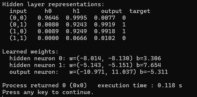
Figure 2-8 prints the representation the hidden layer settled on. The hidden layer outputs will show you what the network discovered. It will not be the same OR and AND split we hand picked. The network finds its own decomposition, whatever makes the math work. The hidden representations are the network’s internal language for describing the problem. Every neural network, from this tiny XOR solver to billion-parameter language models, learns internal representations in its hidden layers. The difference is only scale.
2.10 What Just Happened
Let us step back and name what we built.
Forward pass. Data flows from input through hidden layer to output. Each neuron computes a weighted sum plus bias, then applies sigmoid. We store the intermediate values because the backward pass needs them.
Loss function. We compute MSE between the network’s output and the target. This is a single number that says how wrong the network is.
Backward pass, or backpropagation. The error signal flows from the output back to the hidden layer. At each neuron we compute a delta, which is the upstream error times the local sigmoid derivative. The delta tells us how much to change each weight. We update weights by subtracting the learning rate times the gradient.
Gradient descent. We repeat forward-backward-update for many epochs. Each epoch pushes the weights slightly downhill on the loss surface. Eventually the network finds weights that produce correct outputs.
This is the training loop that every neural network uses. The architecture gets more complex, the loss functions change, the optimizers get smarter, but the core loop of forward, compute loss, backward, update weights and repeat never changes. You could memorize this if you’re that type of person, but I promise as you work though the book you’ll understand this by intuition rather than by having to remember the sequence.
2.11 Key Takeaways
A single perceptron can only solve linearly separable problems. Adding a hidden layer lets the network learn non-linear decision boundaries.
The hidden layer transforms inputs into a new representation where the problem becomes linearly separable. The output layer then solves the transformed problem.
Backpropagation uses the chain rule to compute how much each weight contributed to the error. The gradient flows backward from output to input, one layer at a time.
Each neuron’s delta is the upstream error multiplied by the local sigmoid derivative. delta = upstream * sigmoid_output * (1 - sigmoid_output).
We update weights by subtracting lr * delta * input, which is gradient descent moving us downhill on the loss surface.
The forward pass stores intermediate values (hidden outputs). The backward pass needs them to compute gradients. This is why neural networks use memory proportional to the number of layers.
2.12 Exercises
Change the learning rate to 0.1 and run for 50000 epochs. Compare convergence speed. Then try 10.0. What happens?
Add a third hidden neuron. Does it help? Does it hurt? Does the network still learn XOR?
Print the loss every 100 epochs and observe the learning curve. Where does learning happen fastest? Where does it plateau?
Implement the OR gate with the same two-layer network. It should converge much faster than XOR. Why?
Try initializing all weights to zero instead of random values. What happens and why?
Verify the gradients numerically. For each weight w we compute the following. (loss(w + h) - loss(w - h)) / (2 * h) with h = 0.0001. Compare to the analytical gradient from backpropagation. They should match to several decimal places.
Modify the network to use 3 inputs and train on a 3-input XOR (output 1 when an odd number of inputs are 1). How many hidden neurons do you need?