Overfitting and Regularization
Dropout, weight decay, and early stopping
6.1 What You Will Learn
A network that memorizes the training data instead of learning general patterns is useless because it will fail on any input it has not seen before. In the field the name we give for this is called overfitting. In order to recognize it in neural networks, in this chapter you will see overfitting happen, measure it with a train/validation split, and I’ll teach you the techniques to fight it. The things you will learn in this chapter are very applicable and you will use on every network you build from here on.
6.2 The Problem
A neural network with enough parameters can memorize any dataset perfectly. Give it 100 data points and 1000 weights, and it will find a way to get zero training loss by encoding every example directly. It’s actually an art that comes with experience of choosing a network that’s not so large that it’ll try to memorize your dataset, while not being so small that it can’t learn to generalize well. The problem is that when a network memorizes a dataset, the patterns it learns are noise, not signal. When it sees new data, it produces garbage.
The gap between training performance and real world performance is the generalization gap. Our goal is not zero training loss, it is the smallest possible loss on data the network has never seen, the only way you’ll understand this problem is to watch it in action, so let’s do it!
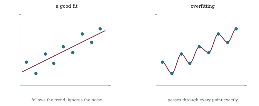
Figure 6-1 shows the two outcomes on the same nine measurements. The left panel follows the trend and leaves every point a little way off, because the points themselves carry noise and a model that honors the noise is honoring something that will not repeat. The right panel passes through all nine exactly, which makes its training loss zero and its usefulness zero with it. Ask the right hand curve about a value between two of its points and it answers with whatever detour it took to reach the next one.
The uncomfortable part is that nothing in the training loss can tell these two apart. The curve on the right scores better by the only number the network is minimizing, which is exactly why the fix has to come from outside the loss.
6.3 A Noisy Dataset
First we need a dataset large enough to split into training and validation sets. We will generate a simple classification problem: points inside a circle are class 1, points outside are class 0. Then we add noise so the boundary is not clean.
/* 033_Noisy_Dataset.c */
#include <stdio.h>
#include <stdlib.h>
#include <math.h>

typedef struct {
    float x[2];
    float t;       /* target: 0 or 1 */
}
Sample;

static float randf(void)
{
    return (float)rand() / RAND_MAX;
}

static void generate_data(Sample *data, int n)
{
    int i;
    for (i = 0; i < n; i++) {
        data[i].x[0] = randf() * 4.0f - 2.0f;
        /* range [-2, 2] */
        data[i].x[1] = randf() * 4.0f - 2.0f;

        float dist = data[i].x[0] * data[i].x[0]
                   + data[i].x[1] * data[i].x[1];

        /* Circle with radius 1.2, plus 20% noise */
        float noise = randf() * 0.4f - 0.2f;
        data[i].t = (dist + noise < 1.44f)
            ? 1.0f
            : 0.0f;
    }
}

int main(void)
{
    Sample data[200];
    int i, c0 = 0, c1 = 0;

    srand(42);
    generate_data(data, 200);

    for (i = 0; i < 200; i++) {
        if (data[i].t > 0.5f) c1++;
        else c0++;
    }

    printf("Generated 200 samples\n");
    printf("  Class 0 (outside): %d\n", c0);
    printf("  Class 1 (inside):  %d\n", c1);
    printf("\nFirst 10 samples:\n");
    for (i = 0; i < 10; i++)
        printf("  (%+6.3f, %+6.3f) -> %.0f\n",
               data[i].x[0], data[i].x[1], data[i].t);

    return 0;
}
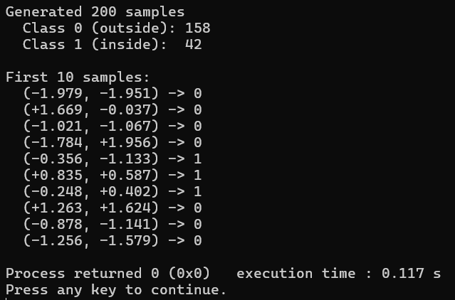
Figure 6-2 is the dataset, two hundred points either side of a noisy circular boundary. The noise means a perfect classifier is impossible because some points near the boundary have the wrong label. A network that memorizes the training set will learn these wrong labels as though they were real patterns.
6.4 Train/Validation Split
Right now on order to setup for overfitting, we split the data: 160 samples for training, 40 for validation. The network never sees the validation set during training. We compute loss on both sets after each epoch and when training loss keeps dropping but validation loss starts rising, the network is overfitting.
/* 034_Overfit.c */
#include <stdio.h>
#include <stdlib.h>
#include <math.h>

static float sigmoid(float z)
{
    return 1.0f / (1.0f + expf(-z));
}
static float randf(void)
{
    return (float)rand() / RAND_MAX;
}

/* 2-input, 20-hidden, 1-output (intentionally
   oversized) */
#define N_HID 20
#define N_PARAMS (2*N_HID + N_HID + N_HID + 1)  /* wh
    + bh + wo + bo */

static float forward(const float *p, const float x[2],
    float h[N_HID])
{
    int i, j;
    /* Hidden layer */
    for (i = 0; i < N_HID; i++) {
        float z = p[2 * N_HID + i];  /* bias */
        for (j = 0; j < 2; j++)
            z += p[i * 2 + j] * x[j];
        h[i] = sigmoid(z);
    }
    /* Output */
    {
        int base_wo = 3 * N_HID;
        float z = p[base_wo + N_HID];  /* output bias */
        for (i = 0; i < N_HID; i++)
            z += p[base_wo + i] * h[i];
        return sigmoid(z);
    }
}

static void backward(const float *p, const float x[2],
    const float h[N_HID],
   float y, float t, float *g)
{
    int i, j;
    int base_bh = 2 * N_HID;
    int base_wo = 3 * N_HID;
    float delta_out = -2.0f * (t - y) * y * (1.0f - y);

    for (i = 0; i < N_PARAMS; i++) g[i] = 0.0f;

    /* Output gradients */
    for (i = 0; i < N_HID; i++)
        g[base_wo + i] = delta_out * h[i];
    g[base_wo + N_HID] = delta_out;

    /* Hidden gradients */
    for (i = 0; i < N_HID; i++) {
        float dh = delta_out * p[base_wo + i] * h[i]
            * (1.0f - h[i]);
        for (j = 0; j < 2; j++)
            g[i * 2 + j] = dh * x[j];
        g[base_bh + i] = dh;
    }
}

typedef struct { float *m, *v; float b1, b2, eps, lr,
    b1t, b2t;
    int n;
    }
    Adam;
static Adam adam_create(int n, float lr) {
    Adam o;
    o.m = (float*)calloc(n, sizeof(float));
    o.v = (float*)calloc(n, sizeof(float));
    o.b1 = 0.9f;
    o.b2 = 0.999f;
    o.eps = 1e-8f;
    o.lr = lr;
    o.b1t = 1;
    o.b2t = 1;
    o.n = n;
    return o;
    }
static void adam_update(Adam *o, float *p,
    const float *g) {
    int i;
    o->b1t *= o->b1;
    o->b2t *= o->b2;
    for(i = 0;i<o->n;i++) {
        o->m[i] = o->b1*o->m[i]+(1-o->b1)*g[i];
        o->v[i] = o->b2*o->v[i]+(1-o->b2)*g[i]*g[i];
        float mh = o->m[i]/(1-o->b1t),
            vh = o->v[i]/(1-o->b2t);
        p[i] -= o->lr*mh/(sqrtf(vh)+o->eps);
        }
        }
static void adam_free(Adam *o)
{
    free(o->m);
    free(o->v);
}

typedef struct { float x[2]; float t; } Sample;

static void generate_data(Sample *data, int n)
{
    int i;
    for (i = 0; i < n; i++) {
        data[i].x[0] = randf() * 4.0f - 2.0f;
        data[i].x[1] = randf() * 4.0f - 2.0f;
        float dist = data[i].x[0]*data[i].x[0]
            + data[i].x[1]*data[i].x[1];
        float noise = randf() * 0.4f - 0.2f;
        data[i].t = (dist + noise < 1.44f)
            ? 1.0f
            : 0.0f;
    }
}

static float eval_loss(const float *p,
    const Sample *data, int n)
{
    float total = 0.0f;
    int i;
    for (i = 0; i < n; i++) {
        float h[N_HID];
        float y = forward(p, data[i].x, h);
        float d = data[i].t - y;
        total += d * d;
    }
    return total / n;
}

int main(void)
{
    Sample data[200];
    float params[N_PARAMS], grads[N_PARAMS],
        grad_acc[N_PARAMS];
    Adam opt;
    int epoch, s, i;

    srand(42);
    generate_data(data, 200);

    /* Initialize params */
    for (i = 0; i < N_PARAMS; i++)
        params[i] = randf() * 0.4f - 0.2f;

    opt = adam_create(N_PARAMS, 0.001f);

    printf("Training 20-hidden network (oversized for "
           "200 samples)\n");
    printf("  epoch   train_loss  val_loss    gap\n");
    for (epoch = 0; epoch < 500; epoch++) {
        /* Train on first 160 samples */
        for (i = 0; i < N_PARAMS; i++)
            grad_acc[i] = 0.0f;
        for (s = 0; s < 160; s++) {
            float h[N_HID];
            float y = forward(params, data[s].x, h);
            backward(params, data[s].x, h, y,
                data[s].t, grads);
            for (i = 0; i < N_PARAMS; i++)
                grad_acc[i] += grads[i];
        }
        for (i = 0; i < N_PARAMS; i++)
            grad_acc[i] /= 160.0f;
        adam_update(&opt, params, grad_acc);

        if ((epoch + 1) % 50 == 0) {
            float tl = eval_loss(params, data, 160);
            float vl = eval_loss(params,
                data + 160, 40);
            printf("  %4d    %.6f    %.6f    %+.6f\n",
                   epoch + 1, tl, vl, vl - tl);
        }
    }

    adam_free(&opt);
    return 0;
}
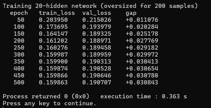
Figure 6-3 has the training loss falling while the validation loss turns back up. Watch the gap column. Early in training, both losses drop together, which means the network is genuinely learning the circle boundary. But at some point, training loss keeps falling while validation loss levels off or starts rising, and that divergence is overfitting. The network has enough capacity to memorize the specific noise in the training samples rather than learning the general shape, and 20 hidden neurons is far more than a simple circle boundary needs, which makes this happen faster.
Training loss never stops improving because the network can always fit the training data more precisely, but validation loss plateaus around epoch 150-200 and then starts creeping back up. That divergence is the signal that tells you when to stop. Everything after roughly epoch 150 is wasted compute that actually makes the model perform worse on data it hasn’t seen before.
6.5 Weight Decay (L2 Regularization)
The first fix for overfitting is weight decay. The core insight is that overfitting networks develop large weights because they need extreme values to carve out the sharp, complex decision boundaries required to memorize individual training samples. If you punish the network for having large weights, it’s forced to find simpler solutions that generalize better. The mechanism is straightforward we add a penalty to the loss function that grows as the weights get bigger. The network is now optimizing two things simultaneously. It wants predictions to be accurate (low data loss) and it wants weights to stay small (low penalty). These two goals compete with each other, and the balance between them is what prevents the network from overfitting without crippling its ability to learn.
The name “weight decay” comes from the effect it has during training. Every update, each weight gets pulled slightly toward zero by the penalty gradient, so unused or unnecessary weights gradually decay away. Only weights that are genuinely earning their keep by reducing the data loss survive, because they need to be large enough that the accuracy benefit outweighs the penalty cost. Look at this formula.
The normal loss function only measures how wrong the predictions are. This adds a second term, we take every weight in the network, square it, add them all up, and multiply by lambda. That sum gets added to the loss. Now the optimizer isn’t just trying to minimize prediction error, it’s also trying to keep the weights small, because big weights increase the total loss. The network has to balance being accurate against being simple, and lambda controls where that balance sits. A large lambda (like 0.01) heavily penalizes big weights and forces the network toward a simpler model, even if it means slightly worse training accuracy. A small lambda (like 0.0001) is a gentle nudge that only kicks in when weights start getting unreasonably large.
Figure 6-4 fits the same nine points twice with the same model, changing only whether that penalty term is present. Without it the fit is free to use whatever weights reach every point, and it does, with a largest coefficient of 766. With the penalty the largest coefficient falls to 2.4 and the curve it produces has nowhere near enough freedom to chase individual points. Neither fit was told to be smooth, and smoothness is not something the penalty measures. It falls out of keeping the weights small, because a wild curve needs large weights to build its swings and the penalty makes those swings expensive.
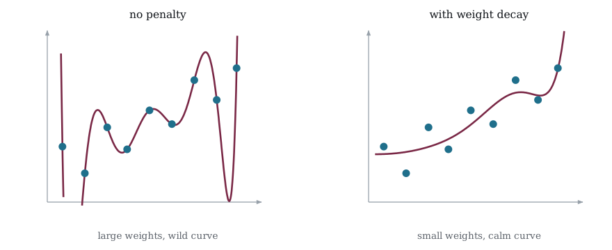
Why does this help with overfitting? When a network memorizes noise, it does so by developing large weights that create sharp, spiky decision boundaries tailored to individual training samples. Penalizing large weights makes those sharp boundaries expensive, so the optimizer settles for smoother, more general solutions that transfer better to unseen data. The name “L2 regularization” comes from linear algebra, where the L2 norm is the square root of the sum of squares. Same idea here, just without the square root since it doesn’t change where the minimum is. Now look at this equation.
This is the derivative of the penalty term with respect to a single weight. The data loss gradient tells the optimizer “move this weight to reduce prediction error.” This penalty gradient says “also move this weight toward zero.” You add them together before the optimizer step, so every weight update has a small force pulling it back toward zero. The strength of that pull is proportional to the weight itself: big weights get pulled harder, small weights barely feel it. The factor of 2 comes from differentiating w^2, same as how the derivative of x^2 is 2x from basic calculus.
/* 035_Weight_Decay.c */
#include <stdio.h>
#include <stdlib.h>
#include <math.h>

static float sigmoid(float z)
{
    return 1.0f / (1.0f + expf(-z));
}
static float randf(void)
{
    return (float)rand() / RAND_MAX;
}

#define N_HID 20
#define N_PARAMS (2*N_HID + N_HID + N_HID + 1)

static float forward(const float *p, const float x[2],
    float h[N_HID])
{
    int i, j;
    for (i = 0; i < N_HID; i++) {
        float z = p[2*N_HID + i];
        for (j = 0; j < 2; j++) z += p[i*2+j] * x[j];
        h[i] = sigmoid(z);
    }
    { int bw = 3*N_HID; float z = p[bw+N_HID];
      for (i = 0; i < N_HID; i++) z += p[bw+i] * h[i];
      return sigmoid(z);
      }
}

static void backward(const float *p, const float x[2],
    const float h[N_HID],
                      float y, float t, float *g)
{
    int i, j, bh = 2*N_HID, bw = 3*N_HID;
    float delta_out = -2.0f * (t - y) * y * (1.0f - y);
    for (i = 0; i < N_PARAMS; i++) g[i] = 0.0f;
    for (i = 0; i < N_HID; i++)
        g[bw+i] = delta_out * h[i];
    g[bw+N_HID] = delta_out;
    for (i = 0; i < N_HID; i++) {
        float dh = delta_out * p[bw+i] * h[i]
            * (1.0f - h[i]);
        for (j = 0; j < 2; j++) g[i*2+j] = dh * x[j];
        g[bh+i] = dh;
    }
}

typedef struct { float *m, *v; float b1, b2, eps, lr,
    b1t, b2t;
    int n;
    }
    Adam;
static Adam adam_create(int n, float lr) {
    Adam o;
    o.m = (float*)calloc(n, sizeof(float));
    o.v = (float*)calloc(n, sizeof(float));
    o.b1 = 0.9f;
    o.b2 = 0.999f;
    o.eps = 1e-8f;
    o.lr = lr;
    o.b1t = 1;
    o.b2t = 1;
    o.n = n;
    return o;
    }
static void adam_update(Adam *o, float *p,
    const float *g) {
    int i;
    o->b1t *= o->b1;
    o->b2t *= o->b2;
    for(i = 0;i<o->n;i++) {
        o->m[i] = o->b1*o->m[i]+(1-o->b1)*g[i];
        o->v[i] = o->b2*o->v[i]+(1-o->b2)*g[i]*g[i];
        float mh = o->m[i]/(1-o->b1t),
            vh = o->v[i]/(1-o->b2t);
        p[i] -= o->lr*mh/(sqrtf(vh)+o->eps);
        }
        }
static void adam_free(Adam *o)
{
    free(o->m);
    free(o->v);
}

typedef struct { float x[2]; float t; } Sample;
static void generate_data(Sample *d, int n) {
    int i;
    for (i = 0;i<n;i++) {
        d[i].x[0] = randf()*4
        -2;
        d[i].x[1] = randf()*4-2;
        float dist = d[i].x[0]*d[i].x[0]
            +d[i].x[1]*d[i].x[1];
        float noise = randf()*0.4f-0.2f;
        d[i].t = (dist+noise<1.44f)?1.0f:0.0f;
        }
        }
static float eval_loss(const float *p,
    const Sample *d, int n) {
    float t = 0;
    int i;
    for(i = 0;i<n;i++) {
        float h[N_HID];
        float y = forward(p, d[i].x, h);
        float diff = d[i].t-y;
        t += diff*diff;
        }
        return t/n;
        }

int main(void)
{
    Sample data[200];
    float params[N_PARAMS], grads[N_PARAMS],
        grad_acc[N_PARAMS];
    Adam opt;
    float lambda = 0.01f;   /* weight decay strength */
    int epoch, s, i;

    srand(42);
    generate_data(data, 200);
    for (i = 0; i < N_PARAMS; i++)
        params[i] = randf() * 0.4f - 0.2f;
    opt = adam_create(N_PARAMS, 0.001f);

    printf("Training with weight decay "
           "(lambda=%.3f)\n", lambda);
    printf("  epoch   train_loss  val_loss    gap\n");
    for (epoch = 0; epoch < 500; epoch++) {
        for (i = 0; i < N_PARAMS; i++)
            grad_acc[i] = 0.0f;
        for (s = 0; s < 160; s++) {
            float h[N_HID];
            float y = forward(params, data[s].x, h);
            backward(params, data[s].x, h, y,
                data[s].t, grads);
            for (i = 0; i < N_PARAMS; i++)
                grad_acc[i] += grads[i];
        }
        for (i = 0; i < N_PARAMS; i++) {
            grad_acc[i] /= 160.0f;
            /* Add weight decay gradient: 2 * lambda
               * w */
            grad_acc[i] += 2.0f * lambda * params[i];
        }
        adam_update(&opt, params, grad_acc);

        if ((epoch + 1) % 50 == 0) {
            float tl = eval_loss(params, data, 160);
            float vl = eval_loss(params,
                data + 160, 40);
            printf("  %4d    %.6f    %.6f    %+.6f\n",
                   epoch + 1, tl, vl, vl - tl);
        }
    }

    /* Print weight magnitudes */
    float sum_sq = 0.0f;
    for (i = 0; i < N_PARAMS; i++)
        sum_sq += params[i] * params[i];
    printf("\nSum of squared weights: %.4f\n", sum_sq);

    adam_free(&opt);
    return 0;
}
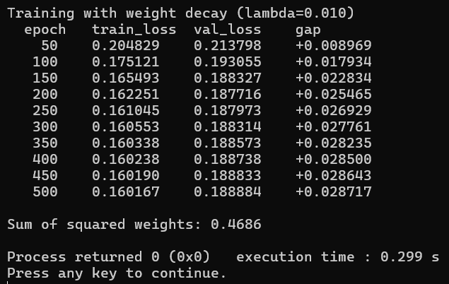
Figure 6-5 reruns the same training with weight decay. Compare the gap column to the run with no penalty at all. The gap here stabilizes around +0.028 and stays there from roughly epoch 250 onward, instead of growing continuously like it did without weight decay. The network has settled into a solution and stopped drifting further from reality. The trade off is visible in the training loss. It floors out around 0.160, which is higher than step 2 achieved because the weight decay penalty prevents the network from cranking its weights up high enough to perfectly fit every training sample. That sounds like a worse result until you look at the validation loss, which sits around 0.188 and stays flat. In step 2, validation loss started climbing back up after epoch 150 as the network memorized noise. Here it plateaus and holds, meaning the model actually works on data it hasn’t seen before.
The sum of squared weights at the bottom (0.4686) confirms the mechanism. Without weight decay, those weights would be much larger because the network has no reason to keep them small. With the penalty active, the optimizer found a solution that uses modest weight values, which produces the smoother decision boundary that generalizes instead of memorizing.
6.6 Dropout
Dropout is a different approach to regularization that works by deliberately breaking the network during training. Each training step, you randomly pick a fraction of the hidden neurons and force their outputs to zero, as if they don’t exist. The next step, you pick a different random set, so the network never knows which neurons will be available, so it can’t rely on any single neuron or any specific combination of neurons to carry the answer. It’s forced to spread the learned information across many neurons redundantly, which produces a more robust model that generalizes better.
During inference, you want the full network available because you’re done training and want the best possible prediction. But there’s a scaling problem, during training, only a fraction of neurons were active at any given time, so the network learned to produce outputs calibrated to that reduced capacity. If you suddenly turn all neurons on at test time, the activations are too large because more neurons are contributing than the network expects. The original dropout paper fixes this by scaling outputs down at inference time by (1 - dropout_rate) to match what the network saw during training. Inverted dropout flips the fix to the training side instead. During training, the surviving neurons get scaled up by 1 / (1 - dropout_rate) so their combined output has the same expected magnitude as if all neurons were active. That way, at inference time you just run the network normally with no special scaling step. Most modern frameworks and libraries use inverted dropout because it keeps the inference path clean, and it’s the approach we’ll implement here.
/* 036_Dropout.c */
#include <stdio.h>
#include <stdlib.h>

static float randf(void)
{
    return (float)rand() / RAND_MAX;
}

/* Inverted dropout: zero out random neurons, scale
   survivors up.
   mask[] stores which neurons were kept (1)
   or dropped (0).
   During inference, skip this function entirely. */

static void dropout(float *h, int *mask,
    int n, float rate)
{
    float scale = 1.0f / (1.0f - rate);
    int i;

    for (i = 0; i < n; i++) {
        if (randf() < rate) {
            h[i] = 0.0f;
            mask[i] = 0;
        }
        else {
            h[i] *= scale;
            mask[i] = 1;
        }
    }
}

int main(void)
{
    float h[10] = { 1.0f, 2.0f, 3.0f, 4.0f, 5.0f,
                    6.0f, 7.0f, 8.0f, 9.0f, 10.0f };
    int mask[10];
    float rate = 0.3f;
    int i;

    srand(42);

    printf("Before dropout:\n  ");
    for (i = 0; i < 10; i++) printf("%.1f ", h[i]);

    dropout(h, mask, 10, rate);

    printf("\n\nAfter dropout (rate=%.1f):\n  ", rate);
    for (i = 0; i < 10; i++) printf("%.1f ", h[i]);

    printf("\n\nMask:\n  ");
    for (i = 0; i < 10; i++) printf("%d ", mask[i]);

    /* Verify: expected value is preserved */
    float sum_before = 55.0f;  /* sum of 1..10 */
    float sum_after = 0.0f;
    for (i = 0; i < 10; i++) sum_after += h[i];
    printf("\n\nSum before: %.1f", sum_before);
    printf("\nSum after:  %.1f (varies by run, but "
           "expected value ~%.1f)\n",
           sum_after, sum_before);

    return 0;
}
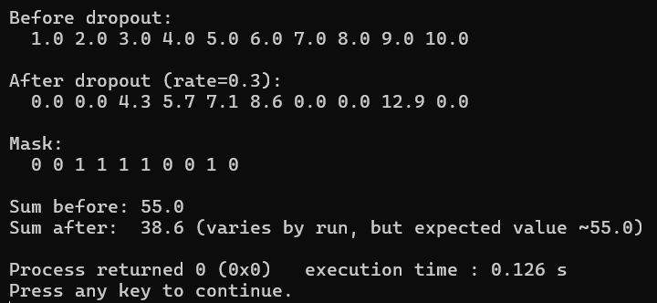
Figure 6-6 has one activation vector before and after dropout, along with the mask and the rescaling. The key insight is the scaling. If we drop 30% of neurons, the remaining 70% are scaled by 1/0.7 = 1.43. This means the expected total activation is the same whether dropout is on or off. The network learns features that are robust to individual neurons being absent. During backpropagation, the mask determines which neurons receive gradients. Dropped neurons get zero gradient. Kept neurons get their gradient scaled by the same 1/(1-rate) factor. We store the mask from the forward pass and reuse it in the backward pass.
6.7 Dropout in the Training Loop
Now let us plug dropout into our overfitting network. We apply dropout to the hidden layer during training and skip it during evaluation.
/* 037_Dropout_Train.c */
#include <stdio.h>
#include <stdlib.h>
#include <math.h>

static float sigmoid(float z)
{
    return 1.0f / (1.0f + expf(-z));
}
static float randf(void)
{
    return (float)rand() / RAND_MAX;
}

#define N_HID 20
#define N_PARAMS (2*N_HID + N_HID + N_HID + 1)

static float forward(const float *p, const float x[2],
    float h[N_HID])
{
    int i, j;
    for (i = 0; i < N_HID; i++) {
        float z = p[2*N_HID + i];
        for (j = 0; j < 2; j++) z += p[i*2+j] * x[j];
        h[i] = sigmoid(z);
    }
    { int bw = 3*N_HID; float z = p[bw+N_HID];
      for (i = 0; i < N_HID; i++) z += p[bw+i] * h[i];
      return sigmoid(z);
      }
}

static void dropout_forward(float *h, int *mask,
    int n, float rate)
{
    float scale = 1.0f / (1.0f - rate);
    int i;
    for (i = 0; i < n; i++) {
        if (randf() < rate) {
            h[i] = 0.0f;
            mask[i] = 0;
            }
        else { h[i] *= scale; mask[i] = 1; }
    }
}

static void backward_with_dropout(const float *p,
    const float x[2],
    const float h[N_HID], const int mask[N_HID],
    float y, float t, float *g, float drop_rate)
{
    int i, j, bh = 2*N_HID, bw = 3*N_HID;
    float delta_out = -2.0f * (t - y) * y * (1.0f - y);
    float scale = 1.0f / (1.0f - drop_rate);

    for (i = 0; i < N_PARAMS; i++) g[i] = 0.0f;

    /* Output layer uses the dropout-modified h
       values */
    for (i = 0; i < N_HID; i++)
        g[bw+i] = delta_out * h[i];
    g[bw+N_HID] = delta_out;

    /* Hidden layer: only update kept neurons */
    for (i = 0; i < N_HID; i++) {
        if (!mask[i]) continue;
        /* dropped neuron: skip */
        /* h[i] already includes the scale factor
           from dropout */
        float h_unscaled = h[i] / scale;
        /* recover original sigmoid output */
        float dh = delta_out * p[bw+i] * h_unscaled
            * (1.0f - h_unscaled);
        dh *= scale;
        /* scale gradient like KANN does */
        for (j = 0; j < 2; j++) g[i*2+j] = dh * x[j];
        g[bh+i] = dh;
    }
}

typedef struct { float *m, *v; float b1, b2, eps, lr,
    b1t, b2t;
    int n;
    }
    Adam;
static Adam adam_create(int n, float lr) {
    Adam o;
    o.m = (float*)calloc(n, sizeof(float));
    o.v = (float*)calloc(n, sizeof(float));
    o.b1 = 0.9f;
    o.b2 = 0.999f;
    o.eps = 1e-8f;
    o.lr = lr;
    o.b1t = 1;
    o.b2t = 1;
    o.n = n;
    return o;
    }
static void adam_update(Adam *o, float *p,
    const float *g) {
    int i;
    o->b1t *= o->b1;
    o->b2t *= o->b2;
    for(i = 0;i<o->n;i++) {
        o->m[i] = o->b1*o->m[i]+(1-o->b1)*g[i];
        o->v[i] = o->b2*o->v[i]+(1-o->b2)*g[i]*g[i];
        float mh = o->m[i]/(1-o->b1t),
            vh = o->v[i]/(1-o->b2t);
        p[i] -= o->lr*mh/(sqrtf(vh)+o->eps);
        }
        }
static void adam_free(Adam *o)
{
    free(o->m);
    free(o->v);
}

typedef struct { float x[2]; float t; } Sample;
static void generate_data(Sample *d, int n) {
    int i;
    for(i = 0;i<n;i++) {
        d[i].x[0] = randf()*4
        -2;
        d[i].x[1] = randf()*4-2;
        float dist = d[i].x[0]*d[i].x[0]
            +d[i].x[1]*d[i].x[1];
        d[i].t = (dist+randf()*0.4f-0.2f<1.44f)
            ?1.0f
            :0.0f;
        }
        }
static float eval_loss(const float *p,
    const Sample *d, int n) {
    float t = 0;
    int i;
    for(i = 0;i<n;i++) {
        float h[N_HID];
        float y = forward(p, d[i].x, h);
        float diff = d[i].t-y;
        t += diff*diff;
        }
        return t/n;
        }

int main(void)
{
    Sample data[200];
    float params[N_PARAMS], grads[N_PARAMS],
        grad_acc[N_PARAMS];
    Adam opt;
    float drop_rate = 0.3f;
    int epoch, s, i;

    srand(42);
    generate_data(data, 200);
    for (i = 0; i < N_PARAMS; i++)
        params[i] = randf() * 0.4f - 0.2f;
    opt = adam_create(N_PARAMS, 0.001f);

    printf("Training with dropout "
           "(rate=%.1f)\n", drop_rate);
    printf("  epoch   train_loss  val_loss    gap\n");
    for (epoch = 0; epoch < 500; epoch++) {
        for (i = 0; i < N_PARAMS; i++)
            grad_acc[i] = 0.0f;
        for (s = 0; s < 160; s++) {
            float h[N_HID];
            int mask[N_HID];
            float y;

            /* Forward with dropout (training mode) */
            forward(params, data[s].x, h);
            dropout_forward(h, mask, N_HID, drop_rate);

            /* Recompute output with dropped hidden
               values */
            { int bw = 3
                *N_HID;
                float z = params[bw+N_HID];
              for (i = 0; i < N_HID; i++)
                  z += params[bw+i] * h[i];
              y = sigmoid(z);
              }

            backward_with_dropout(params,
                data[s].x, h, mask,
                                   y, data[s].t,
                    grads, drop_rate);
            for (i = 0; i < N_PARAMS; i++)
                grad_acc[i] += grads[i];
        }
        for (i = 0; i < N_PARAMS; i++)
            grad_acc[i] /= 160.0f;
        adam_update(&opt, params, grad_acc);

        if ((epoch + 1) % 50 == 0) {
            /* Eval without dropout */
            float tl = eval_loss(params, data, 160);
            float vl = eval_loss(params,
                data + 160, 40);
            printf("  %4d    %.6f    %.6f    %+.6f\n",
                   epoch + 1, tl, vl, vl - tl);
        }
    }

    adam_free(&opt);
    return 0;
}
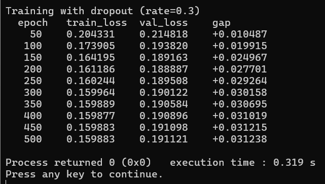
Figure 6-7 puts dropout in the training loop, and the gap settles instead of widening. Compare it to the run with no regularization at all. The gap here settles around +0.031 and holds steady, rather than growing without bound as the network memorizes training data. The validation loss lands around 0.191 and stays flat from epoch 200 onward, which means the network has found a solution that works on unseen data and isn’t drifting away from it.
The mechanism is different from weight decay even though the result looks similar. Weight decay kept the weights small so the decision boundary stayed smooth. Dropout does something more aggressive: it randomly removes neurons during every training step, so the network can never build a solution that depends on any specific neuron being present. If neuron 7 has learned to recognize a particular training sample, that’s useless when neuron 7 gets dropped. The network is forced to spread that knowledge across multiple neurons so the answer is still approximately correct even with a random subset missing. The redundancy this creates is what makes the model robust at inference time when all neurons are active.
Notice the training loss (0.159) is almost identical to what weight decay achieved (0.160), and the validation loss is slightly higher (0.191 vs 0.188). On this particular problem, weight decay performed marginally better, but that’s not a general rule. Dropout tends to shine more on larger networks with many layers, where individual neurons are more likely to co-adapt and memorize together. On a single hidden layer with 20 neurons, both techniques end up in roughly the same place.
6.8 Early Stopping
The simplest regularization technique requires no code changes to the network at all. Just stop training when the validation loss starts rising. Save the weights at the best validation loss and use those. In practice I will use this method a lot, train the model, save weights every few epochs and then validate until the optimum point is reached.
/* 038_Early_Stopping.c */
#include <stdio.h>
#include <stdlib.h>
#include <math.h>
#include <string.h>

static float sigmoid(float z)
{
    return 1.0f / (1.0f + expf(-z));
}
static float randf(void)
{
    return (float)rand() / RAND_MAX;
}

#define N_HID 20
#define N_PARAMS (2*N_HID + N_HID + N_HID + 1)

static float forward(const float *p, const float x[2],
    float h[N_HID])
{
    int i, j;
    for (i = 0; i < N_HID; i++) {
        float z = p[2*N_HID + i];
        for (j = 0; j < 2; j++) z += p[i*2+j] * x[j];
        h[i] = sigmoid(z);
    }
    { int bw = 3*N_HID; float z = p[bw+N_HID];
      for (i = 0; i < N_HID; i++) z += p[bw+i] * h[i];
      return sigmoid(z);
      }
}

static void backward(const float *p, const float x[2],
    const float h[N_HID],
                      float y, float t, float *g)
{
    int i, j, bh = 2*N_HID, bw = 3*N_HID;
    float delta_out = -2.0f * (t - y) * y * (1.0f - y);
    for (i = 0; i < N_PARAMS; i++) g[i] = 0.0f;
    for (i = 0; i < N_HID; i++)
        g[bw+i] = delta_out * h[i];
    g[bw+N_HID] = delta_out;
    for (i = 0; i < N_HID; i++) {
        float dh = delta_out * p[bw+i] * h[i]
            * (1.0f - h[i]);
        for (j = 0; j < 2; j++) g[i*2+j] = dh * x[j];
        g[bh+i] = dh;
    }
}

typedef struct { float *m, *v; float b1, b2, eps, lr,
    b1t, b2t;
    int n;
    }
    Adam;
static Adam adam_create(int n, float lr) {
    Adam o;
    o.m = (float*)calloc(n, sizeof(float));
    o.v = (float*)calloc(n, sizeof(float));
    o.b1 = 0.9f;
    o.b2 = 0.999f;
    o.eps = 1e-8f;
    o.lr = lr;
    o.b1t = 1;
    o.b2t = 1;
    o.n = n;
    return o;
    }
static void adam_update(Adam *o, float *p,
    const float *g) {
    int i;
    o->b1t *= o->b1;
    o->b2t *= o->b2;
    for(i = 0;i<o->n;i++) {
        o->m[i] = o->b1*o->m[i]+(1-o->b1)*g[i];
        o->v[i] = o->b2*o->v[i]+(1-o->b2)*g[i]*g[i];
        float mh = o->m[i]/(1-o->b1t),
            vh = o->v[i]/(1-o->b2t);
        p[i] -= o->lr*mh/(sqrtf(vh)+o->eps);
        }
        }
static void adam_free(Adam *o)
{
    free(o->m);
    free(o->v);
}

typedef struct { float x[2]; float t; } Sample;
static void generate_data(Sample *d, int n) {
    int i;
    for(i = 0;i<n;i++) {
        d[i].x[0] = randf()*4
        -2;
        d[i].x[1] = randf()*4-2;
        float dist = d[i].x[0]*d[i].x[0]
            +d[i].x[1]*d[i].x[1];
        d[i].t = (dist+randf()*0.4f-0.2f<1.44f)
            ?1.0f
            :0.0f;
        }
        }
static float eval_loss(const float *p,
    const Sample *d, int n) {
    float t = 0;
    int i;
    for(i = 0;i<n;i++) {
        float h[N_HID];
        float y = forward(p, d[i].x, h);
        float diff = d[i].t-y;
        t += diff*diff;
        }
        return t/n;
        }

int main(void)
{
    Sample data[200];
    float params[N_PARAMS], grads[N_PARAMS],
        grad_acc[N_PARAMS];
    float best_params[N_PARAMS];
    Adam opt;
    float best_val = 1e30f;
    int best_epoch = 0;
    int patience = 50, streak = 0;
    int epoch, s, i;

    srand(42);
    generate_data(data, 200);
    for (i = 0; i < N_PARAMS; i++)
        params[i] = randf() * 0.4f - 0.2f;
    opt = adam_create(N_PARAMS, 0.001f);

    printf("Training with early stopping "
           "(patience=%d)\n", patience);
    printf("  epoch   train_loss  val_loss    best_val "
           "  status\n");
    for (epoch = 0; epoch < 1000; epoch++) {
        for (i = 0; i < N_PARAMS; i++)
            grad_acc[i] = 0.0f;
        for (s = 0; s < 160; s++) {
            float h[N_HID];
            float y = forward(params, data[s].x, h);
            backward(params, data[s].x, h, y,
                data[s].t, grads);
            for (i = 0; i < N_PARAMS; i++)
                grad_acc[i] += grads[i];
        }
        for (i = 0; i < N_PARAMS; i++)
            grad_acc[i] /= 160.0f;
        adam_update(&opt, params, grad_acc);

        float vl = eval_loss(params, data + 160, 40);

        if (vl < best_val) {
            best_val = vl;
            best_epoch = epoch + 1;
            memcpy(best_params, params, sizeof(params));
            streak = 0;
        }
        else {
            streak++;
        }

        if ((epoch + 1) % 50 == 0) {
            float tl = eval_loss(params, data, 160);
            printf("  %4d    %.6f    %.6f    %.6f   "
                   "%s\n",
                   epoch + 1, tl, vl, best_val,
            streak > 0 ? "waiting..."
                       : "new best");
        }

        if (streak >= patience) {
            printf("\n  Early stop at epoch %d. Best "
                   "was epoch %d.\n",
                   epoch + 1, best_epoch);
            break;
        }
    }

    /* Restore best weights */
    memcpy(params, best_params, sizeof(params));
    float final_tl = eval_loss(params, data, 160);
    float final_vl = eval_loss(params, data + 160, 40);
    printf("\n  Restored best weights (epoch "
           "%d)\n", best_epoch);
    printf("  Final train_loss=%.6f  val_loss=%.6f\n",
        final_tl, final_vl);

    adam_free(&opt);
    return 0;
}
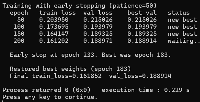
Figure 6-8 has early stopping firing on patience and restoring the best weights. The patience parameter controls how many epochs without improvement we tolerate before stopping. Setting it too low risks stopping before the network has fully trained. Setting it too high risks wasting compute on overfitting. 50 is a reasonable default.
6.9 Using Them Together
In practice you combine all three techniques. Weight decay and dropout fight overfitting during training. Early stopping catches any remaining overfitting by stopping at the right time. A typical recipe.
Weight decay lambda = 1e-4 to 1e-3
Dropout rate = 0.1 to 0.5 (higher for larger networks)
Early stopping with patience = 10 to 50 epochs
You tune these based on the gap between training and validation loss. If the gap is large, increase regularization. If training loss is high (underfitting), decrease regularization.
6.10 Key Takeaways
Overfitting is when the network memorizes training data instead of learning general patterns. It shows as a gap between training loss and validation loss.
Always split your data into training and validation sets. The validation set is your ground truth for generalization.
Weight decay adds a penalty proportional to the sum of squared weights. It pushes the network toward smaller, smoother solutions. Implemented by adding 2 * lambda * w_i to each gradient.
Dropout randomly zeros out hidden neurons during training and scales survivors by 1/(1-rate). This forces redundant representations. During inference, dropout is turned off. KANN stores a mask and scales by the same factor in the backward pass.
Early stopping saves the weights at the lowest validation loss and stops training when validation loss has not improved for a set number of epochs.
These techniques trade a small increase in training loss for a larger decrease in validation loss. The goal is never to minimize training loss. It is to minimize validation loss.
6.11 Exercises
Run 034_Overfit.c for 2000 epochs instead of 500. How bad does the gap get? Plot (or print) training and validation loss to see the divergence.
Try different weight decay values: 0.1, 0.01, 0.001, 0.0001. Which gives the smallest validation loss? Which causes underfitting?
Try different dropout rates. 0.1, 0.3, 0.5, 0.7. At what rate does the network start underfitting (training loss stays high)?
Combine weight decay and dropout in one training loop. Does the combination work better than either alone?
Reduce the hidden layer from 20 to 4 neurons and train without any regularization. Does overfitting still occur? This is the simplest regularization: use a smaller network.
Implement L1 regularization (penalty = lambda * sum(|w_i|), gradient = lambda * sign(w_i)). How does it differ from L2 in the learned weight distribution?