Gradient Descent and Optimizers
SGD, momentum, RMSprop, and Adam
5.1 What You Will Learn
Every network we have trained so far has used the same rule, which subtracts the learning rate multiplied by the gradient from each weight. That rule is vanilla gradient descent and it has carried us a long way, but it treats a difficult loss surface exactly the same as an easy one. It crawls where the surface is flat, it thrashes where the surface is a narrow valley, and it applies one learning rate to every weight in the network whether that weight sits on a steep slope or a gentle one.
An optimizer is what we put in place of that rule. It sits between the gradients that backpropagation produces and the weights those gradients are meant to change, and it decides how much of each gradient to actually apply. Nothing about the forward pass changes and nothing about the backward pass changes, so everything built in the previous chapters still holds. What changes is the single line that turns a gradient into an update.
In this chapter you will build four optimizers from scratch, watching each one fix a specific failure of the one before it. Momentum carries a running average of past gradients so that a consistent direction builds speed. RMSprop gives every weight its own effective learning rate based on how large its gradients have been. Adam combines both ideas and adds a correction for the bias those running averages carry at the start of training. By the end you will have a reusable optimizer module that the rest of the book uses.
5.2 The Problem with Vanilla SGD
Before we can improve on the rule we have to be specific about how it fails, and the failures are easier to see on a surface simple enough to picture than inside a network with thousands of parameters. Stochastic gradient descent updates each weight with a single line.
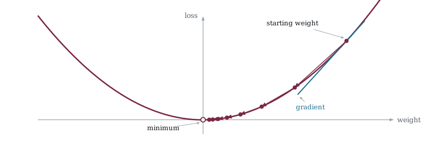
Figure 5-1 is that one line drawn out for a single weight. The curve is the loss as that weight varies, the tangent is the gradient where the weight currently sits, and subtracting a fraction of it moves the weight downhill toward the minimum. Notice that each step is shorter than the one before it even though the learning rate never changes, because the slope itself flattens as the weight approaches the bottom and a smaller slope produces a smaller correction. That self limiting behavior is the reason the plain rule works at all, and it is also the reason it becomes so slow near a minimum.
This works, but this has three problems. First, the same learning rate applies to every weight so weights with large gradients get huge updates while weights with tiny gradients barely move. Secondly, the update is purely local, so it only looks at the current gradient and has no memory of what happened in previous steps. Third, in flat regions of the loss surface the gradient is near zero and training stalls, even though the minimum might be just past the flat region.
The learning rate decides how far each of those steps goes, and neither extreme works.
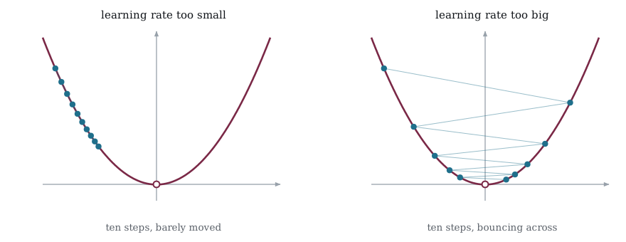
Both panels of Figure 5-2 run ten steps from the same starting weight on the same curve, and the only difference is the size of the step. On the left the rate is small enough that ten steps barely leave the starting point, so the answer is right and arrives too late to be useful. On the right the rate overshoots the bottom on every step and lands on the far side, so the weight bounces across the minimum instead of settling into it. Push that rate a little higher and the bounces grow rather than shrink, at which point training diverges and the loss runs off to infinity.
Let us make these problems visible by optimizing a simple 2D function instead of a neural network, so we can watch the path the optimizer takes.
/* 026_SGD.c */
#include <stdio.h>

/* A bowl-shaped function: f(x,y) = x^2 + 10*y^2
   Minimum is at (0, 0).
   The y-direction is 10x steeper than x, creating
   a narrow valley that causes SGD to zigzag. */

static void gradient(float x, float y, float *gx, float *gy)
{
    *gx = 2.0f * x;
    *gy = 20.0f * y;
}

int main(void)
{
    float x = 5.0f, y = 3.0f;
    float lr = 0.05f;
    int i;

    printf("Vanilla SGD on f(x,y) = x^2 + 10*y^2\n");
    printf("  step   x        y        f(x,y)\n");
    for (i = 0; i < 30; i++) {
        float f = x * x + 10.0f * y * y;
        if (i % 5 == 0)
            printf("  %3d   %+7.4f  %+7.4f  %8.4f\n", i, x,
                y, f);

        float gx, gy;
        gradient(x, y, &gx, &gy);
        x -= lr * gx;
        y -= lr * gy;
    }
    float f = x * x + 10.0f * y * y;
    printf("  %3d   %+7.4f  %+7.4f  %8.4f\n", 30, x, y, f);
    return 0;
}
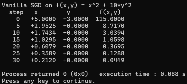
Figure 5-3 sends vanilla SGD zigzagging down the narrow valley. Watch x and y converge. The y coordinate oscillates because the gradient in y is 10 times larger than in x, but the learning rate is the same for both. If you increase the learning rate to speed up x, y will diverge. If you decrease it to stabilize y, x will crawl. There is no single learning rate that works well for both directions. This is the fundamental problem with vanilla SGD.
5.3 Momentum
The first improvement is to give the optimizer memory. Instead of using only the current gradient, we keep a running average of past gradients called the velocity. The update becomes.
The velocity v is a running total that remembers past gradients. Each step you take the old velocity; we shrink it by multiplying by beta (which is usually around 0.9, meaning we keep 90% of what we knew), then we add the new gradient on top. First step, v is just the gradient. Second step, it’s 90% of the first gradient plus the new one. Third step, 90% of that sum plus the newest gradient. Old gradients fade exponentially but never fully disappear. If the gradient keeps pointing the same direction for many steps, v grows larger and larger in that direction. If the gradient keeps flipping sign (positive, negative, positive, negative), the additions cancel each other out and v stays small. Which leads us to again look at this formula.
Instead of stepping by the raw gradient, you step by the velocity. This is the same SGD update rule from before, but with v replacing the gradient. When v has built up because gradients were consistent, the step is bigger than any single gradient would have produced. When v is small because gradients were oscillating, the step is smaller. The network automatically takes big confident steps in directions it’s sure about and cautious steps in directions where the signal is noisy.
Think of it like a ball rolling downhill. It builds up speed on consistent slopes and its inertia carries it through small bumps and flat regions.
/* 027_Momentum.c */
#include <stdio.h>

static void gradient(float x, float y, float *gx, float *gy)
{
    *gx = 2.0f * x;
    *gy = 20.0f * y;
}

int main(void)
{
    float x = 5.0f, y = 3.0f;
    float lr = 0.05f;
    float beta = 0.9f;
    float vx = 0.0f, vy = 0.0f;   /* velocity */
    int i;

    printf("SGD with Momentum on f(x,y) = x^2 + 10*y^2\n");
    printf("  step   x        y        f(x,y)\n");
    for (i = 0; i < 30; i++) {
        float f = x * x + 10.0f * y * y;
        if (i % 5 == 0)
            printf("  %3d   %+7.4f  %+7.4f  %8.4f\n", i, x,
                y, f);

        float gx, gy;
        gradient(x, y, &gx, &gy);

        vx = beta * vx + gx;
        vy = beta * vy + gy;

        x -= lr * vx;
        y -= lr * vy;
    }
    float f = x * x + 10.0f * y * y;
    printf("  %3d   %+7.4f  %+7.4f  %8.4f\n", 30, x, y, f);
    return 0;
}
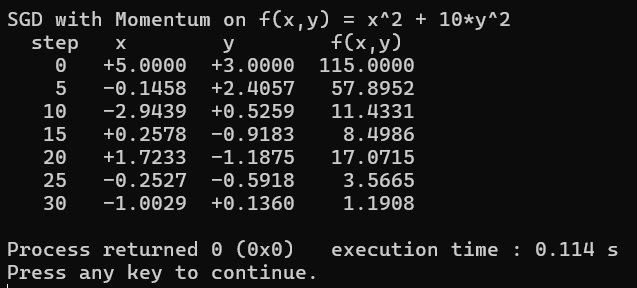
Figure 5-4 shows momentum has a problem that vanilla SGD doesn’t have in that it overshoots. Look at step 15, where f(x,y) drops to 8.49, then at step 20 it jumps back up to 17.07. The ball rolled past the bottom of the valley and climbed up the other side. Vanilla SGD never does that because it has no memory, so it can’t build up too much speed.
But look at the overall trend. It starts at 115 and by step 30 it’s down to 1.19. The overshooting gets smaller each time because the velocity dampens as the gradients start pointing against the direction of travel. The ball bounces back and forth but each bounce is smaller than the last, like a marble settling into a bowl. Compare this to where vanilla SGD is at step 30 and you’ll see momentum got closer to the minimum despite the wobble. It traded a smooth path for a faster arrival.
5.4 RMSprop
Momentum remembers which direction to go but still takes the same size step for every weight. If one gradient is consistently huge and another is consistently tiny, they both get scaled by the same learning rate. That’s the different-scales problem, but RMSprop fixes this by tracking how big each weight’s gradient has been. The variable r is a running average of the squared gradient. Squaring makes everything positive, so it measures magnitude regardless of direction. The decay parameter (typically 0.999) controls how far back the memory goes, same idea as beta in momentum. Look at this formula.
This line keeps a running average of how big the gradient has been. Each step, you keep most of the old average (decay is typically 0.999, so 99.9% of the old value stays) and mix in a small fraction of the new gradient squared. The squaring makes everything positive so negative and positive gradients both contribute to the magnitude. After many steps, r settles into a measure of “how active has this weight been.” A weight that’s been getting large gradients has a large r. A weight with small gradients has a small r. Which brings us to the other formula.
This is the SGD update with one change, the learning rate is divided by sqrt(r + epsilon) before being multiplied by the gradient. If r is large (the weight has been getting big gradients), sqrt(r) is large, the division shrinks the step, and the weight moves cautiously. If r is small (the weight has been getting tiny gradients), sqrt(r) is small, the division barely shrinks anything, and the weight takes a relatively bigger step. The epsilon (typically 1e-8) is just a safety guard so you never divide by zero. It has no effect on the math otherwise.
The result is that every weight in the network gets it own automatically tuned learning rate, computed from its own gradient history. There is no manual tuning per layer so there is no guessing.
/* 028_RMSPROP.c */
#include <stdio.h>
#include <math.h>

static void gradient(float x, float y, float *gx, float *gy)
{
    *gx = 2.0f * x;
    *gy = 20.0f * y;
}

int main(void)
{
    float x = 5.0f, y = 3.0f;
    float lr = 0.1f;
    float decay = 0.9f;
    float eps = 1e-6f;
    float rx = 0.0f, ry = 0.0f;
    /* running avg of squared gradients */
    int i;

    printf("RMSprop on f(x,y) = x^2 + 10*y^2\n");
    printf("  step   x        y        f(x,y)\n");
    for (i = 0; i < 30; i++) {
        float f = x * x + 10.0f * y * y;
        if (i % 5 == 0)
            printf("  %3d   %+7.4f  %+7.4f  %8.4f\n", i, x,
                y, f);

        float gx, gy;
        gradient(x, y, &gx, &gy);

        rx = decay * rx + (1.0f - decay) * gx * gx;
        ry = decay * ry + (1.0f - decay) * gy * gy;

        x -= lr / sqrtf(rx + eps) * gx;
        y -= lr / sqrtf(ry + eps) * gy;
    }
    float f = x * x + 10.0f * y * y;
    printf("  %3d   %+7.4f  %+7.4f  %8.4f\n", 30, x, y, f);
    return 0;
}
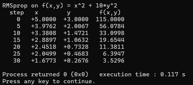
Figure 5-5 brings both coordinates down at the same rate. Notice that x and y converge at similar rates even though the raw gradients in y are 10 times larger. RMSprop automatically compensates for the difference in scale. The y direction has large gradients, so ry is large, and the effective learning rate for y is reduced. The x direction has small gradients, so rx is small, and the effective learning rate for x is boosted. Look at the path: every single step, f(x,y) decreases there is no overshooting like momentum, no zigzag like vanilla SGD. It goes 115, 56, 33, 19, 11, 6, 3.5 which is a smooth descent every time. That’s the payoff of per-weight learning rates.
But notice it’s at 3.5 after 30 steps, the momentum was at 1.19. RMSprop is smoother but slower here because it lacks momentum’s ability to build up speed in a consistent direction. So we are not in a predicament, it solved the scaling problem but lost the acceleration. However, there is a way to get around this, we can use an optimizer called Adam, which combines both.
5.5 Adam
Adam (Adaptive Moment Estimation) combines the two ideas you just saw. Momentum tracks which direction the gradients have been pointing. RMSprop tracks how large they’ve been, however Adam does both at the same time. It keeps two running averages per weight. The first moment m is the average gradient, same concept as velocity in momentum. The second moment v is the average squared gradient, same concept as r in RMSprop. Both use their own decay rates: beta1 (typically 0.9) for the first moment, beta2 (typically 0.999) for the second.
There’s one extra piece that momentum and RMSprop didn’t bother with: bias correction. Both m and v start at zero, which means for the first few steps they’re biased toward zero simply because the running average hasn’t had time to warm up. Adam fixes this by dividing each moment by (1 - beta^t) where t is the step number. Early on, when t is small, this divisor is small, which scales the moments up to compensate. After a few hundred steps the correction factor approaches 1 and effectively disappears. It’s a startup fix, nothing more. The final update divides the corrected first moment by the square root of the corrected second moment. Direction from momentum, scaling from RMSprop, startup fix from bias correction. That’s why Adam is the default optimizer in most training code. It’s not the best at any one thing, but it handles almost everything reasonably well without much tuning. We need to break this down to understand what it is doing, and we can start with the first of the four lines that make it up.
This is momentum’s velocity under a different name. Keep 90% of the old average (beta1 = 0.9), mix in 10% of the new gradient. After many steps, m represents the average direction the gradient has been pointing. If gradients consistently point one way, m is large in that direction. If they oscillate, m stays small.
This is RMSprop’s r under a different name. Keep 99.9% of the old average (beta2 = 0.999), mix in 0.1% of the new gradient squared. After many steps, v represents how large the gradients have been for this weight. The longer decay rate means it has a longer memory than m, so it’s a more stable estimate of gradient magnitude.
Bias correction for the first moment. At step 1, m is just 10% of one gradient, which underestimates the true average. Dividing by (1 - 0.9^1) = 0.1 scales it back up by 10x. By step 10, (1 - 0.9^10) = 0.65, so the correction is small. By step 100 it’s basically 1.0 and does nothing. This just fixes the cold start.
Same correction for the second moment, except that beta2 is 0.999 so the warmup takes longer. At step 1, (1 - 0.999^1) = 0.001, so it scales up by 1000x. This sounds extreme but v at step 1 is just 0.1% of one squared gradient, so the correction is accurate.
The actual weight update. The numerator m_hat is the momentum direction: where to go. The denominator sqrt(v_hat) + epsilon is the RMSprop scaling: how cautiously to step. Weights with large noisy gradients have large v_hat, so the denominator is large, so the step is small. Weights with consistent small gradients have small v_hat, so the step is relatively larger. The epsilon (1e-8) prevents division by zero, nothing more.
Let’s see this in action.
/* 029_ADAM.c */
#include <stdio.h>
#include <math.h>

static void gradient(float x, float y, float *gx, float *gy)
{
    *gx = 2.0f * x;
    *gy = 20.0f * y;
}

int main(void)
{
    float x = 5.0f, y = 3.0f;
    float lr = 0.1f;
    float beta1 = 0.9f, beta2 = 0.999f;
    float eps = 1e-8f;
    float mx = 0.0f, my = 0.0f;    /* first moment */
    float vx = 0.0f, vy = 0.0f;    /* second moment */
    float b1t = 1.0f, b2t = 1.0f;
    /* beta1^t, beta2^t for bias correction */
    int i;

    printf("Adam on f(x,y) = x^2 + 10*y^2\n");
    printf("  step   x        y        f(x,y)\n");
    for (i = 0; i < 30; i++) {
        float f = x * x + 10.0f * y * y;
        if (i % 5 == 0)
            printf("  %3d   %+7.4f  %+7.4f  %8.4f\n", i, x,
                y, f);

        float gx, gy;
        gradient(x, y, &gx, &gy);

        /* Update moments */
        mx = beta1 * mx + (1.0f - beta1) * gx;
        my = beta1 * my + (1.0f - beta1) * gy;
        vx = beta2 * vx + (1.0f - beta2) * gx * gx;
        vy = beta2 * vy + (1.0f - beta2) * gy * gy;

        /* Bias correction */
        b1t *= beta1;
        b2t *= beta2;
        float mx_hat = mx / (1.0f - b1t);
        float my_hat = my / (1.0f - b1t);
        float vx_hat = vx / (1.0f - b2t);
        float vy_hat = vy / (1.0f - b2t);

        /* Update parameters */
        x -= lr * mx_hat / (sqrtf(vx_hat) + eps);
        y -= lr * my_hat / (sqrtf(vy_hat) + eps);
    }
    float f = x * x + 10.0f * y * y;
    printf("  %3d   %+7.4f  %+7.4f  %8.4f\n", 30, x, y, f);
    return 0;
}
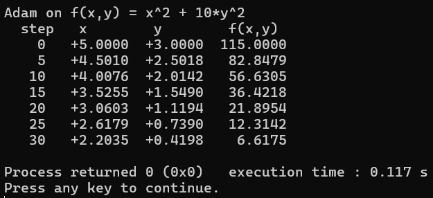
Figure 5-6 has Adam converging without the oscillation either method showed alone, because it combines the best of both, momentum’s ability to build speed in consistent directions and RMSprop’s ability to adapt the learning rate per-parameter. It converges smoothly with minimal oscillation, descending as cleanly as RMSprop did while never overshooting the way momentum did. Every step, f(x,y) decreases through 115, 82, 56, 36, 21, 12 and finally 6.6, without any of the bouncing back up we saw earlier.
That last number is worth sitting with though, because 6.6 after 30 steps puts Adam behind momentum at 1.19 and behind RMSprop at 3.5, making it the slowest of the three on this particular problem, which might seem like a bad result for the optimizer that’s supposed to be the best of both worlds.
The reason is that this toy problem is too simple to show Adam’s strengths. It’s a clean 2D bowl with perfect gradients and no noise. Momentum thrives here because there’s nothing to be cautious about, Adam’s careful per-weight scaling and bias correction are overhead on a problem this clean, like wearing a seatbelt on a bicycle. Adam wins on real networks where you have thousands of weights with wildly different gradient scales, noisy mini-batches, saddle points, and flat regions. The same conservatism that slows it down here is what keeps it stable when training a transformer with millions of parameters. That’s why it’s the default in virtually every deep learning framework despite not winning this 30-step toy race.
5.6 All Four Side by Side
By this point you may have forgotten what the other optimizers look like, so what we’ll do is we’ll run all four optimizers on the same problem with the same starting point and compare convergence.
/* 030_All_Optimizers_Comparison.c */
#include <stdio.h>
#include <math.h>

static void grad(float x, float y, float *gx, float *gy)
{
    *gx = 2.0f * x;
    *gy = 20.0f * y;
}

static float f(float x, float y)
{
    return x*x + 10.0f*y*y;
}

int main(void)
{
    int i;
    float gx, gy;

    /* SGD */
    {
        float x = 5.0f, y = 3.0f, lr = 0.05f;
        for (i = 0; i < 50; i++) {
            grad(x, y, &gx, &gy);
            x -= lr * gx;
            y -= lr * gy;
        }
        printf("SGD        after 50 steps: "
               "f=%.6f  x=%+.6f y=%+.6f\n",
               f(x,y), x, y);
    }

    /* Momentum */
    {
        float x = 5.0f, y = 3.0f, lr = 0.05f, beta = 0.9f;
        float vx = 0, vy = 0;
        for (i = 0; i < 50; i++) {
            grad(x, y, &gx, &gy);
            vx = beta*vx + gx;
            vy = beta*vy + gy;
            x -= lr * vx;
            y -= lr * vy;
        }
        printf("Momentum   after 50 steps: "
               "f=%.6f  x=%+.6f y=%+.6f\n",
               f(x,y), x, y);
    }

    /* RMSprop */
    {
        float x = 5.0f, y = 3.0f, lr = 0.1f;
        float decay = 0.9f, eps = 1e-6f;
        float rx = 0, ry = 0;
        for (i = 0; i < 50; i++) {
            grad(x, y, &gx, &gy);
            rx = decay*rx + (1-decay)*gx*gx;
            ry = decay*ry + (1-decay)*gy*gy;
            x -= lr / sqrtf(rx + eps) * gx;
            y -= lr / sqrtf(ry + eps) * gy;
        }
        printf("RMSprop    after 50 steps: "
               "f=%.6f  x=%+.6f y=%+.6f\n",
               f(x,y), x, y);
    }

    /* Adam */
    {
        float x = 5.0f, y = 3.0f, lr = 0.1f;
        float b1 = 0.9f, b2 = 0.999f, eps = 1e-8f;
        float mx = 0, my = 0, vx = 0, vy = 0;
        float b1t = 1, b2t = 1;
        for (i = 0; i < 50; i++) {
            grad(x, y, &gx, &gy);
            mx = b1*mx + (1-b1)*gx;
            my = b1*my + (1-b1)*gy;
            vx = b2*vx + (1-b2)*gx*gx;
            vy = b2*vy + (1-b2)*gy*gy;
            b1t *= b1;
            b2t *= b2;
            float mxh = mx/(1-b1t), myh = my/(1-b1t);
            float vxh = vx/(1-b2t), vyh = vy/(1-b2t);
            x -= lr * mxh / (sqrtf(vxh) + eps);
            y -= lr * myh / (sqrtf(vyh) + eps);
        }
        printf("Adam       after 50 steps: "
               "f=%.6f  x=%+.6f y=%+.6f\n",
               f(x,y), x, y);
    }

    return 0;
}
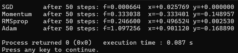
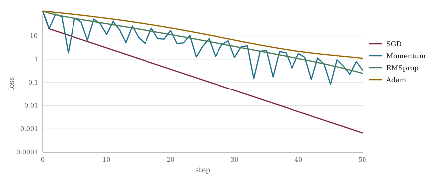
Figure 5-8 plots the loss at every step of those same four runs rather than only the final number, on a logarithmic scale because the values span five orders of magnitude and a linear axis would press everything below 1 flat against the baseline. The shape of each curve says more than its endpoint does, and the one to look at is momentum, which oscillates the whole way down around the smooth line RMSprop walks.
Figure 5-7 is the table of final positions after fifty steps, and the numbers speak for themselves. Compare how close each optimizer gets to f = 0 (the minimum) after the same number of steps. SGD wins on this toy function because the y-gradient is so steep it converges that dimension immediately, while the adaptive optimizers are still warming up their moment estimates. On real networks with thousands of parameters and complex loss surfaces, Adam dominates.
5.7 A Reusable Optimizer
Let us package Adam into a reusable module. This is the optimizer you will use for the rest of the book. It works on a flat array of parameters, which is how real networks store their weights.
/* 031_Reusable_Optimizer.c */
#include <stdio.h>
#include <stdlib.h>
#include <math.h>

typedef struct {
    float *m;       /* first moment (mean of gradients) */
    float *v;
    /* second moment (mean of squared gradients) */
    float beta1;
    float beta2;
    float eps;
    float lr;
    float b1t;      /* beta1^t for bias correction */
    float b2t;      /* beta2^t for bias correction */
    int n;          /* number of parameters */
} Adam;

static Adam adam_create(int n, float lr)
{
    Adam opt;
    opt.m = (float *)calloc(n, sizeof(float));
    opt.v = (float *)calloc(n, sizeof(float));
    opt.beta1 = 0.9f;
    opt.beta2 = 0.999f;
    opt.eps = 1e-8f;
    opt.lr = lr;
    opt.b1t = 1.0f;
    opt.b2t = 1.0f;
    opt.n = n;
    return opt;
}

static void adam_update(Adam *opt, float *params,
    const float *grads)
{
    int i;
    opt->b1t *= opt->beta1;
    opt->b2t *= opt->beta2;

    for (i = 0; i < opt->n; i++) {
        opt->m[i] = opt->beta1 * opt->m[i]
            + (1.0f - opt->beta1) * grads[i];
        opt->v[i] = opt->beta2 * opt->v[i]
            + (1.0f - opt->beta2) * grads[i] * grads[i];

        float m_hat = opt->m[i] / (1.0f - opt->b1t);
        float v_hat = opt->v[i] / (1.0f - opt->b2t);

        params[i] -= opt->lr * m_hat
            / (sqrtf(v_hat) + opt->eps);
    }
}

static void adam_free(Adam *opt)
{
    free(opt->m);
    free(opt->v);
    opt->m = NULL;
    opt->v = NULL;
}

/* --- Test on our 2D function --- */

int main(void)
{
    float params[2] = { 5.0f, 3.0f };
    /* x and y as a parameter array */
    float grads[2];
    Adam opt = adam_create(2, 0.1f);
    int i;

    printf("Adam optimizer module test\n");
    printf("  step   x        y        f(x,y)\n");
    for (i = 0; i < 50; i++) {
        float fval = params[0]*params[0] + 10.0f*params[1]
            *params[1];
        if (i % 10 == 0)
            printf("  %3d   %+7.4f  %+7.4f  %8.4f\n", i,
                params[0], params[1], fval);

        grads[0] = 2.0f * params[0];
        grads[1] = 20.0f * params[1];
        adam_update(&opt, params, grads);
    }
    float fval = params[0]*params[0] + 10.0f*params[1]
        *params[1];
    printf("  %3d   %+7.4f  %+7.4f  %8.4f\n", 50, params[0],
        params[1], fval);

    adam_free(&opt);
    return 0;
}
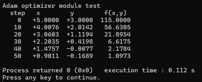
Figure 5-9 runs the same Adam training behind a create, update and free interface. The adam_create/adam_update/adam_free pattern is the same create/use/destroy pattern you use for any resource in C. The params and grads are flat arrays. You compute the gradients however you want (backpropagation), then call adam_update with the parameter array and the gradient array. The optimizer handles everything else.
This is the interface we will use going forward. For every network we build in later chapters, the training loop will be: forward pass, compute loss, backward pass to fill the gradient array, call adam_update, repeat.
5.8 Plugging Into XOR
Let us swap our manual SGD updates from Chapter 2 with the Adam optimizer and train XOR again. This shows the optimizer module working on an actual neural network.
/* 032_XOR_ADAM.c */
#include <stdio.h>
#include <stdlib.h>
#include <math.h>

/* --- Adam optimizer (from step 6) --- */

typedef struct {
    float *m, *v;
    float beta1, beta2, eps, lr, b1t, b2t;
    int n;
} Adam;

static Adam adam_create(int n, float lr) {
    Adam o;
    o.m = (float*)calloc(n, sizeof(float));
    o.v = (float*)calloc(n, sizeof(float));
    o.beta1 = 0.9f;
    o.beta2 = 0.999f;
    o.eps = 1e-8f;
    o.lr = lr;
    o.b1t = 1.0f;
    o.b2t = 1.0f;
    o.n = n;
    return o;
    }
static void adam_update(Adam *o, float *p, const float *g) {
    int i;
    o->b1t *= o->beta1;
    o->b2t *= o->beta2;
    for (i = 0; i<o->n; i++) { o->m[i] = o->beta1*o->m[i]
        +(1-o->beta1)*g[i]; o->v[i] = o->beta2*o->v[i]
        +(1-o->beta2)*g[i]*g[i];
        float mh = o->m[i]/(1-o->b1t), vh = o->v[i]
            /(1-o->b2t);
        p[i] -= o->lr*mh/(sqrtf(vh)+o->eps);
        } }
static void adam_free(Adam *o)
{
    free(o->m);
    free(o->v);
}

/* --- Network stored as flat arrays --- */

/* Layout: wh[0][0], wh[0][1], wh[1][0],
   wh[1][1], bh[0], bh[1],
           wo[0], wo[1], bo
   Total: 9 parameters */

static float sigmoid(float z)
{
    return 1.0f / (1.0f + expf(-z));
}

static float forward(const float *p, const float x[2],
    float h[2])
{
    int i, j;
    /* Hidden layer: p[0..3] = weights, p[4..5] = biases */
    for (i = 0; i < 2; i++) {
        float z = p[4 + i];  /* bias */
        for (j = 0; j < 2; j++)
            z += p[i * 2 + j] * x[j];
        h[i] = sigmoid(z);
    }
    /* Output: p[6..7] = weights, p[8] = bias */
    {
        float z = p[8];
        for (i = 0; i < 2; i++)
            z += p[6 + i] * h[i];
        return sigmoid(z);
    }
}

static void backward(const float *p, const float x[2],
    const float h[2],
                      float y, float t, float *g)
{
    int i, j;
    float delta_out = -2.0f * (t - y) * y * (1.0f - y);
    float delta_h[2];

    for (i = 0; i < 2; i++)
        delta_h[i] = delta_out * p[6 + i] * h[i]
            * (1.0f - h[i]);

    /* Zero gradient buffer */
    for (i = 0; i < 9; i++) g[i] = 0.0f;

    /* Output gradients */
    for (i = 0; i < 2; i++)
        g[6 + i] = delta_out * h[i];
    g[8] = delta_out;

    /* Hidden gradients */
    for (i = 0; i < 2; i++) {
        for (j = 0; j < 2; j++)
            g[i * 2 + j] = delta_h[i] * x[j];
        g[4 + i] = delta_h[i];
    }
}

int main(void)
{
    float X[4][2] = { {0, 0}, {0, 1}, {1, 0}, {1, 1} };
    float T[4] = { 0, 1, 1, 0 };
    float params[9], grads[9];
    Adam opt;
    int epoch, s, i;

    srand(42);
    for (i = 0; i < 9; i++)
        params[i] = ((float)rand() / RAND_MAX) * 2.0f
            - 1.0f;

    opt = adam_create(9, 0.01f);

    for (epoch = 0; epoch < 3000; epoch++) {
        float total_loss = 0.0f;
        float grad_accum[9] = {0};

        for (s = 0; s < 4; s++) {
            float h[2], y, diff;
            y = forward(params, X[s], h);
            diff = T[s] - y;
            total_loss += diff * diff;
            backward(params, X[s], h, y, T[s], grads);
            for (i = 0; i < 9; i++)
                grad_accum[i] += grads[i];
        }

        /* Average gradients over batch */
        for (i = 0; i < 9; i++)
            grad_accum[i] /= 4.0f;

        adam_update(&opt, params, grad_accum);

        if ((epoch + 1) % 500 == 0)
            printf("epoch %4d  loss=%.6f\n", epoch + 1,
                total_loss / 4.0f);
    }

    printf("\nFinal results:\n");
    for (s = 0; s < 4; s++) {
        float h[2];
        float y = forward(params, X[s], h);
        printf("  %.0f XOR %.0f = %.4f  (target %.0f)\n",
               X[s][0], X[s][1], y, T[s]);
    }

    adam_free(&opt);
    return 0;
}
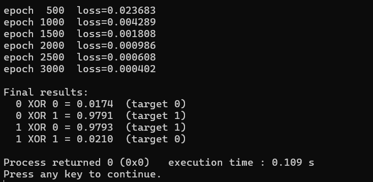
Figure 5-10 trains XOR with Adam over a flat array of nine parameters. Two things to notice. First, the network parameters are stored as a flat array of 9 floats instead of separate struct fields. This is how real frameworks store parameters, as one contiguous block that the optimizer can iterate over. Second, we accumulate gradients across all 4 samples and average them before updating. This is batch gradient descent. In later chapters with larger datasets we will use mini-batches (a subset of the data per update).
5.9 When to Use What
SGD. Almost never on its own. Occasionally useful with momentum for very large models where memory is tight (Adam needs 2x the memory of the parameters for its moment estimates).
SGD + Momentum. A solid choice when you can afford to tune the learning rate carefully. Some researchers still prefer it for training CNNs because it can generalize slightly better than Adam in some cases.
RMSprop. Simple, effective, fewer hyperparameters than Adam (no bias correction). Good for RNNs and problems where the gradient statistics change over time.
Adam. The default. Use this unless you have a specific reason not to. beta1 = 0.9, beta2 = 0.999, epsilon = 1e-8 almost never need tuning. Only the learning rate needs adjustment, and typical values are 0.001 for most networks or 0.0001 for transformers.
For the rest of this book we use Adam.
5.10 Key Takeaways
Vanilla SGD uses a single learning rate for all parameters. It is slow and oscillates when gradient magnitudes differ across dimensions.
Momentum adds memory by keeping a running average of past gradients. It accelerates in consistent directions and dampens oscillation.
RMSprop adapts the learning rate per-parameter by dividing by the running RMS of past gradients. Parameters with large gradients get smaller updates.
Adam combines momentum and RMSprop with bias correction. It is the default optimizer for most neural networks.
Store network parameters as a flat array. The optimizer iterates over the array without knowing the network architecture. This separation is how real frameworks work.
Adam needs 2x the memory of the parameters for its m and v arrays. On an embedded system, this matters.
5.11 Exercises
Run 030_All_Optimizers_Comparison.c with 200 steps instead of 50. Which optimizer reaches the smallest f value?
Change the function to f(x,y) = x^2 + 100*y^2 (even more anisotropic). How does each optimizer handle the increased scale difference?
Implement Nesterov momentum. compute the gradient at the “lookahead” position (w + beta*v) instead of the current position. Does it converge faster on the test function?
Try different learning rates for Adam on XOR: 0.1, 0.01, 0.001, 0.0001. What is the sweet spot?
Measure peak memory usage for each optimizer. SGD needs 0 extra floats per parameter. Momentum needs 1. RMSprop needs 1. Adam needs 2. For a network with 1 million parameters, how many extra bytes does each optimizer require?
Read the RMSprop implementation in KANN (kann.c, search for kann_RMSprop). It has an SSE-optimized path and a scalar fallback. Compare the scalar path to your 028_RMSPROP.c implementation.