Convolution and Filters
1D and 2D convolution, kernels, stride, and padding
8.1 What You Will Learn
So far, every network we have built treats each input feature as completely independent from every other. If the input has 100 features, the network assigns a separate weight to each one and has no idea that feature 5 is next to feature 6 or that feature 50 is far away from feature 3. The position and arrangement of the data is invisible to the network. For signals and images, that arrangement matters enormously. A spike in a sensor reading means the same thing whether it shows up at sample 10 or sample 500 or the edge in a photograph is the same pattern whether it appears in the top left corner or the bottom right. These kinds of patterns are local and they are translation invariant, meaning they do not change their meaning when they shift position.
Convolution exploits exactly this property. Instead of assigning a separate weight to every input, it slides a small filter across the data and applies the same weights at every position, looking for the same pattern everywhere. This means the network only has to learn what a pattern looks like once, and it can detect that pattern no matter where it appears. In this chapter we will build one dimensional and two dimensional convolutions from scratch, and by the end you will understand every parameter involved.
8.2 The Idea
Imagine you have a sensor signal that is 100 samples long and you want to detect sharp spikes in it. One approach is to feed all 100 samples into a multilayer perceptron and hope the network figures out on its own that it should check every position for spikes. That works, but the network has to learn the same spike pattern independently at every position, which means a lot of redundant weights and a lot of wasted training time. The other approach is to define a small spike-detecting filter, say 3 samples wide, and slide it across the signal one position at a time. At each position you multiply the 3 filter values by the 3 signal values underneath, sum them up, and write down the result. The filter has 3 weights instead of 100 and it applies the same weights at every position. If there is a spike anywhere in the signal, the filter will respond strongly when it reaches that spot. This is convolution.
The small filter is called a kernel.
The operation of sliding it across the input and computing a weighted sum at each position is a convolution. The output is a new signal, the same length as the input or close to it, where each value tells you how strongly the kernel’s pattern matched at that location. A high value means the local region of the input looked like the pattern the kernel is searching for. A low value means it did not.
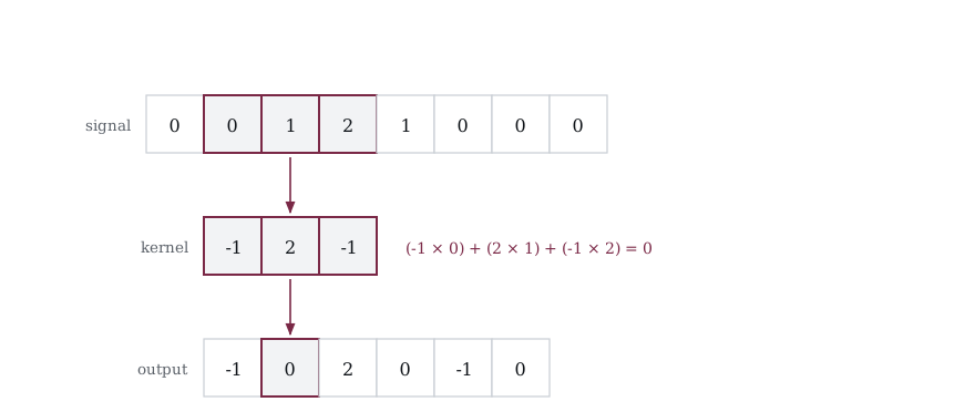
Figure 8-1 freezes the operation at a single position, using the signal and kernel from the first program in this chapter. Three values of the signal sit under the three weights of the kernel, each pair is multiplied, and the three products are added to give one number in the output. Then the kernel moves one place to the right and the same nine keystrokes happen again. That is the whole operation, and everything else in the chapter is a variation on where the kernel lands and how many kernels there are.
Notice that the output is shorter than the input. Eight samples with a kernel of three leaves six positions, because the kernel needs three values under it and runs out of room at each end. We get that length back with padding a little further on.
Let us build it.
8.3 A 1D Convolution by Hand
Start with the simplest case. A signal of 8 values and a kernel of 3 values. The kernel slides across the signal one position at a time. At each position, we multiply the kernel values by the signal values under it and sum the products.
/* 044_1D_Convolution.c */
#include <stdio.h>

int main(void)
{
    /* A simple signal */
    float signal[] = {0, 0, 1, 2, 1, 0, 0, 0};
    int sig_len = 8;

    /* A spike-detecting kernel */
    float kernel[] = { -1, 2, -1};
    int ker_len = 3;

    /* Output length = sig_len - ker_len + 1 */
    int out_len = sig_len - ker_len + 1;
    float output[6];
    int i, k;

    /* convolution: slide kernel across signal */
    for (i = 0; i < out_len; i++)
    {
        float sum = 0.0f;
        for (k = 0; k < ker_len; k++)
            sum += signal[i + k] * kernel[k];

        output[i] = sum;
    }

    printf("Signal: ");
    for (i = 0; i < sig_len; i++)
        printf("%5.1f ", signal[i]);

    printf("\nKernel: ");
    for (k = 0; k < ker_len; k++)
        printf("%5.1f ",kernel[k]);

    printf("\nOutput: ");
    for (i = 0; i < out_len; i++)
        printf("%5.1f ", output[i]);
    printf("\n");


    return 0;
}
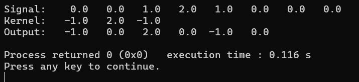
Figure 8-2 slides a three tap kernel across an eight sample signal. The kernel {-1, 2, −1} is a peak detector. It responds strongly wherever the signal rises and then falls, which is exactly what a spike looks like. You can see this in the output: position 2 has a value of 2.0, which is the highest response. That corresponds to the signal values {1, 2, 1} at positions 2, 3, and 4. The math is −11 + 22 + −1*1 = 2. The center sample is high and the neighbors are lower, so the kernel fires.
Look at the rest of the output. Position 0 gives −1.0 because the signal is {0, 0, 1}, which is a rising edge, not a peak. Position 3 gives 0.0 because the signal is {2, 1, 0}, a falling slope with no sharp center. The kernel responds to the shape of the local neighborhood, not to absolute values. The output has 6 values even though the input has 8. That is because a kernel of width 3 needs at least 3 samples to work with, so it cannot start computing until position 0 and has to stop before it runs off the end. The formula is output_length = input_length - kernel_length + 1, which gives 8 - 3 + 1 = 6. The output shrinks by 2 compared to the input. We will deal with this later using padding.
If you have ever written an FIR filter on a microcontroller, this is the same operation. You slide a set of coefficients across a signal and compute a weighted sum at each position. The only difference in a neural network is that the coefficients are not hand-chosen. The network learns them through backpropagation, just like it learns any other weight.
8.4 Multiple Kernels
One kernel detects one pattern. A spike detector does not help you find smooth ramps or oscillations. In a neural network we use multiple kernels, each detecting a different feature. The output of each kernel is called a channel or feature map.
/* 045_Multi_Kernels.c */
#include <stdio.h>

#define SIG_LEN 8
#define KER_LEN 3
#define N_KERNELS 3
#define OUT_LEN (SIG_LEN - KER_LEN + 1)

int main(void)
{
    float signal[SIG_LEN] = { 0, 0, 1, 2, 1, 0, 0, 0 };

    /* Three different kernels */
    float kernels[N_KERNELS][KER_LEN] = {
        { -1,  2, -1 },   /* spike detector */
        {  1,  1,  1 },   /* smoother (average) */
        { -1,  0,  1 },   /* edge detector (rising) */
    };
    const char *names[] = { "spike", "smooth", "edge" };

    float output[N_KERNELS][OUT_LEN];
    int f, i, k;

    /* Apply each kernel */
    for (f = 0; f < N_KERNELS; f++) {
        for (i = 0; i < OUT_LEN; i++) {
            float sum = 0.0f;
            for (k = 0; k < KER_LEN; k++)
                sum += signal[i + k] * kernels[f][k];
            output[f][i] = sum;
        }
    }

    printf("Signal:  ");
    for (i = 0; i < SIG_LEN; i++)
        printf("%5.1f ", signal[i]);
    printf("\n\n");

    for (f = 0; f < N_KERNELS; f++) {
        printf("%-6s:  ", names[f]);
        for (i = 0; i < OUT_LEN; i++)
            printf("%5.1f ", output[f][i]);
        printf("\n");
    }

    return 0;
}
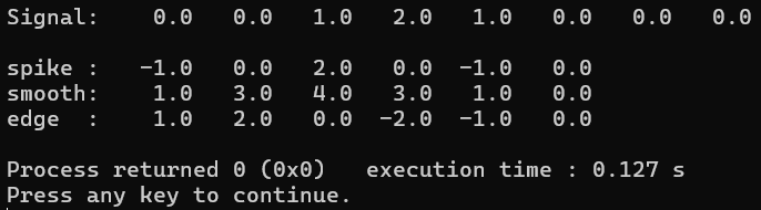
Figure 8-3 has three kernels reading that same signal and reporting different things. Each kernel extracts something different from the same signal. The spike detector {-1, 2, −1} peaks at 2.0 where the signal hits its maximum, the same behavior we saw in 044_1D_Convolution.c. The smoother {1, 1, 1} adds up three neighboring values at each position, producing a blurred version of the signal where the sharp spike at position 2 has been spread out into a gentler bump. Its highest response is 4.0 at position 2, which is just 1 + 2 + 1. The edge detector {-1, 0, 1} responds to rising slopes, hitting 2.0 at position 1 where the signal is climbing from 0 toward 2, and dropping to −2.0 at position 3 where the signal is falling from 2 back down. The three output rows are called feature maps. Each one is a different view of the same input, highlighting a different local property. One sees peaks, one sees averages, one sees slopes. Together they give a much richer description of the signal than any single kernel could provide on its own.
In this example we chose the kernels by hand because we already knew what patterns to look for. In a trained neural network, the kernels are learned through backpropagation just like any other weight. The network starts with random kernel values and the training process gradually shapes them into whatever local patterns are most useful for the task. A network trained on audio might learn kernels that detect pitch changes. A network trained on images might learn kernels that detect edges at specific orientations. The point is that you do not have to design the filters yourself. You define the architecture, how many kernels, how wide, and the network figures out what to put in them.
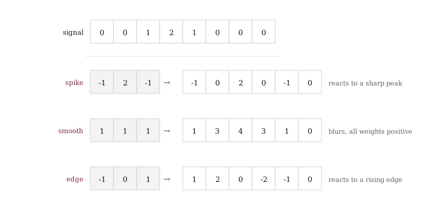
Figure 8-4 runs all three kernels from that program across the same eight samples. Nothing about the signal changes between the three rows and nothing about the sliding changes either, so every difference in the output comes from the three weights. The spike kernel answers loudest at the sharp peak, the smoother answers with a broad hump because all of its weights are positive and it can never cancel anything out, and the edge kernel answers with a positive value on the way up and a negative one on the way down. A convolutional layer holds many kernels for exactly this reason, since each one is a different question asked of the same data.
8.5 Stride
So far the kernel moves one position at a time, computing a weighted sum at every possible location along the signal. The stride parameter controls how far the kernel jumps between positions. With a stride of 1, the kernel checks every position and produces the full output we have been seeing. With a stride of 2, the kernel skips every other position, so it computes at position 0, then position 2, then position 4, and so on. The effect is that the output gets shorter. A stride of 2 roughly halves the output length, and a stride of 3 cuts it to a third. The formula becomes output_length = (input_length - kernel_length) / stride + 1. You lose spatial resolution because you are sampling fewer positions, but you gain efficiency because there are fewer multiplications to do and fewer values for the next layer to process.
The tradeoff is the same. you reduce the amount of data you have to deal with, but you might miss fine details between the samples you skipped.
/* 046_Stride.c */
#include <stdio.h>

static int conv1d(const float *signal, int sig_len,
                  const float *kernel, int ker_len,
                  int stride, float *output)
{
    int out_len = (sig_len - ker_len) / stride + 1;
    int i, k;

    for (i = 0; i < out_len; i++) {
        float sum = 0.0f;
        int start = i * stride;
        for (k = 0; k < ker_len; k++)
            sum += signal[start + k] * kernel[k];
        output[i] = sum;
    }
    return out_len;
}

int main(void)
{
    float signal[] = { 1, 2, 3, 4, 5, 6, 7, 8, 9, 10 };
    int sig_len = 10;
    float kernel[] = { 1, 1, 1 };
    int ker_len = 3;
    float output[10];
    int out_len, i;

    printf("Signal: ");
    for (i = 0; i < sig_len; i++)
        printf("%.0f ", signal[i]);
    printf("\nKernel: 1 1 1 (sum of 3)\n\n");

    out_len = conv1d(signal, sig_len, kernel,
        ker_len, 1, output);
    printf("Stride 1 (%d outputs): ", out_len);
    for (i = 0; i < out_len; i++)
        printf("%.0f ", output[i]);

    out_len = conv1d(signal, sig_len, kernel,
        ker_len, 2, output);
    printf("\nStride 2 (%d outputs): ", out_len);
    for (i = 0; i < out_len; i++)
        printf("%.0f ", output[i]);

    out_len = conv1d(signal, sig_len, kernel,
        ker_len, 3, output);
    printf("\nStride 3 (%d outputs): ", out_len);
    for (i = 0; i < out_len; i++)
        printf("%.0f ", output[i]);

    printf("\n");
    return 0;
}
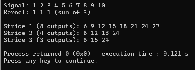
Figure 8-5 runs the same kernel at stride 1, 2 and 3, and reports the output length each one gives. The kernel {1, 1, 1} sums three consecutive values, so the output at each position is just the sum of the three samples underneath. With stride 1, the kernel checks every position and produces 8 outputs. With stride 2, it jumps two positions between each computation and produces 4 outputs. With stride 3, it jumps three and produces only 3. You can verify this: stride 2 gives {6, 12, 18, 24}, which are the sums starting at positions 0, 2, 4, and 6 of the signal. The values at positions 1, 3, and 5 are simply never computed.
The output length formula with stride is output_length = (input_length - kernel_length) / stride + 1. For stride 2 that gives (10 - 3) / 2 + 1 = 4, which matches. For stride 3 it gives (10 - 3) / 3 + 1 = 3, which also matches.
Larger strides are one of the ways neural networks downsample as they go deeper. Instead of computing a response at every position and then throwing some away, the network just skips positions during the convolution itself. This cuts the output size and reduces the amount of computation the next layer has to do. The tradeoff is resolution. A stride of 1 catches everything, while a stride of 2 might miss a feature that falls between two sample points. In practice, networks handle this by using enough kernels at each layer that the important patterns get caught even at reduced resolution.
8.6 Padding
Convolution shrinks the output because the kernel cannot extend past the edges of the signal. A kernel of width 3 on a signal of length 8 gives only 6 outputs, and the deeper you stack convolution layers, the more the signal shrinks at each stage. Sometimes you want the output to be the same length as the input, especially when you are building networks with many layers and you need to control exactly how and when the dimensions change. Padding solves this by adding zeros around the input before the convolution runs, giving the kernel room to operate at the edges without running off the end.
The most common approach is called “same” padding, which adds just enough zeros so that the output length equals the input length when the stride is 1. For a kernel of width 3, that means one zero on each side of the signal. For a kernel of width 5, you need two zeros on each side. The general formula is pad = (kernel_length - 1) / 2 on each side. The padded zeros do not add real information, they are just telling the network “there is nothing here,” but they let the kernel center itself on the very first and very last samples of the signal, which means the edges of the input get the same treatment as the middle.
/* 047_Padding.c */
#include <stdio.h>
#include <string.h>

static int conv1d_padded(const float *signal,
    int sig_len,
                          const float *kernel,
                              int ker_len,
                          int stride, int pad,
                              float *output)
{
    int padded_len = sig_len + 2 * pad;
    int out_len = (padded_len - ker_len) / stride + 1;
    int i, k;

    /* We do not actually allocate a padded array.
       Instead,
      we handle the boundaries in the
      inner loop. */
    for (i = 0; i < out_len; i++) {
        float sum = 0.0f;
        int start = i * stride - pad;
        for (k = 0; k < ker_len; k++) {
            int idx = start + k;
            if (idx >= 0 && idx < sig_len)
                sum += signal[idx] * kernel[k];
            /* else: padded zero, contributes nothing */
        }
        output[i] = sum;
    }
    return out_len;
}

int main(void)
{
    float signal[] = { 1, 2, 3, 4, 5, 6, 7, 8 };
    int sig_len = 8;
    float kernel[] = { 1, 1, 1 };
    int ker_len = 3;
    float output[10];
    int out_len, i;

    printf("Signal (len=%d): ", sig_len);
    for (i = 0; i < sig_len; i++)
        printf("%.0f ", signal[i]);

    printf("\n\nNo padding:     ");
    out_len = conv1d_padded(signal, sig_len, kernel,
        ker_len, 1, 0, output);
    printf("(%d outputs) ", out_len);
    for (i = 0; i < out_len; i++)
        printf("%.0f ", output[i]);

    printf("\nPad=1 ('same'):  ");
    out_len = conv1d_padded(signal, sig_len, kernel,
        ker_len, 1, 1, output);
    printf("(%d outputs) ", out_len);
    for (i = 0; i < out_len; i++)
        printf("%.0f ", output[i]);

    printf("\n\nWith padding, output length = input "
           "length.\n");
    printf("Edge values are smaller because some "
           "kernel positions\n");
    printf("overlap with the zero-padded region.\n");

    return 0;
}
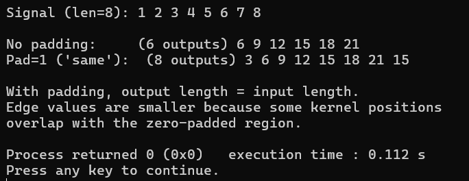
Figure 8-6 runs the same convolution with and without a zero added at each end. Without padding, the 8 input values produce only 6 outputs because the kernel cannot center itself on the first or last sample without hanging off the edge. With pad=1, a zero is added to each end of the signal before the convolution runs, and the output comes back at 8 values, matching the input length exactly.
Look at the difference between the two rows. The middle values are identical: 9, 12, 15, 18 appear in both. But the padded version has 3 at the start and 15 at the end, which are lower than you might expect. That is because at those positions, part of the kernel is sitting on top of the padded zeros. The first output in the padded version is 01 + 11 + 2*1 = 3 instead of what would be 6 if there were real data to the left. The kernel is doing honest math, but one of its three inputs is a zero that we invented. This is the tradeoff with padding: you get to keep the spatial dimensions intact through the layer, but the values at the edges are slightly weaker because the kernel is partially operating on empty space rather than real signal.
8.7 2D Convolution
Images are two dimensional, so the convolution has to work in two dimensions as well. Instead of sliding a kernel along a single row of samples, a 2D kernel slides across both rows and columns of the image. At each position the kernel sits on top of a small rectangular patch of pixels, every element of the kernel gets multiplied by the pixel underneath it, and all the products get summed into a single output value. The math is identical to what we have been doing in 1D, just extended to cover a grid instead of a line.
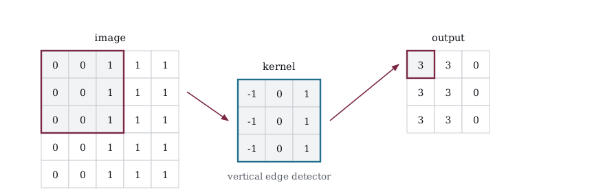
Figure 8-7 shows the same idea one dimension up, with the image, kernel and output from the 2D program. The kernel sits over a square window rather than a run of samples, and the nine products are summed into a single output value exactly as before. The image is deliberately simple, a block of zeros beside a block of ones, and the kernel is a vertical edge detector, so the output finds the boundary between them and reports nothing anywhere else.
A 3x3 kernel on an image means 9 multiplications and one sum at every position. The kernel moves one column at a time across each row, and one row at a time down the image, computing the weighted sum at each stop. The output is a new 2D array, smaller than the input by the same shrinkage rule we saw before, where each value tells you how strongly the kernel’s pattern matched at that location. In 1D we were detecting spikes and edges in a signal. In 2D the same idea applies, but now the patterns are things like horizontal edges, vertical edges, corners, or texture gradients, depending on what values the kernel contains.
/* 048_2D_Convolution.c */
#include <stdio.h>

#define IMG_H 5
#define IMG_W 5
#define KER_H 3
#define KER_W 3
#define OUT_H (IMG_H - KER_H + 1)
#define OUT_W (IMG_W - KER_W + 1)

int main(void)
{
    /* A small "image" with a vertical edge */
    float image[IMG_H][IMG_W] = {
        { 0, 0, 1, 1, 1 },
        { 0, 0, 1, 1, 1 },
        { 0, 0, 1, 1, 1 },
        { 0, 0, 1, 1, 1 },
        { 0, 0, 1, 1, 1 },
    };

    /* Vertical edge detector */
    float kernel[KER_H][KER_W] = {
        { -1, 0, 1 },
        { -1, 0, 1 },
        { -1, 0, 1 },
    };

    float output[OUT_H][OUT_W];
    int oi, oj, ki, kj;

    /* 2D convolution */
    for (oi = 0; oi < OUT_H; oi++) {
        for (oj = 0; oj < OUT_W; oj++) {
            float sum = 0.0f;
            for (ki = 0; ki < KER_H; ki++)
                for (kj = 0; kj < KER_W; kj++)
                    sum += image[oi + ki][oj + kj]
                        * kernel[ki][kj];
            output[oi][oj] = sum;
        }
    }

    printf("Image:\n");
    for (oi = 0; oi < IMG_H; oi++) {
        printf("  ");
        for (oj = 0; oj < IMG_W; oj++)
            printf("%5.1f ", image[oi][oj]);
        printf("\n");
    }

    printf("\nKernel (vertical edge detector):\n");
    for (ki = 0; ki < KER_H; ki++) {
        printf("  ");
        for (kj = 0; kj < KER_W; kj++)
            printf("%5.1f ", kernel[ki][kj]);
        printf("\n");
    }

    printf("\nOutput:\n");
    for (oi = 0; oi < OUT_H; oi++) {
        printf("  ");
        for (oj = 0; oj < OUT_W; oj++)
            printf("%5.1f ", output[oi][oj]);
        printf("\n");
    }

    printf("\nThe edge appears as a column of 3s where "
           "the\n");
    printf("transition from 0 to 1 occurs in the "
           "image.\n");

    return 0;
}
Figure 8-8 finds the column where the image changes. The vertical edge detector kernel has −1 on the left column, 0 in the center, and 1 on the right column, repeated across all three rows. What it computes at each position is essentially the horizontal difference: it subtracts the pixel values on the left side of the patch from the pixel values on the right side. If the left and right sides are the same, those values cancel out and the output is zero. If the image transitions from dark to light as you move left to right, the right side is larger than the left side and the output is positive.
In this example, the image is all zeros on the left two columns and all ones on the right three columns. The edge sits between columns 1 and 2. When the kernel lands on that transition, it sees −10 + 01 + 1*1 on each row, which sums to 3 across the three rows. When the kernel sits entirely on the flat region of zeros or the flat region of ones, the left and right sides are equal and the output is 0. The result is a column of 3s in the output exactly where the vertical edge is in the image, with zeros everywhere else. If you have done any image processing on a microcontroller, this kernel should look familiar. Sobel filters, Prewitt operators, and sharpening masks are all just hand-chosen 2D kernels applied through the same convolution operation. The only difference in a convolutional neural network is that nobody chooses the kernel values. The network starts with random values and backpropagation shapes them into whatever local patterns are most useful for the task, whether that is edges, corners, textures, or something more abstract that a human would never think to look for.
8.8 Putting It All Together
Let us build a proper 1D convolution function with support for multiple input channels, multiple output channels (kernels), stride, padding, and bias. This is the building block for convolutional neural networks.
/* 049_Convolutional_Layer.c */
#include <stdio.h>
#include <math.h>

/* 1D convolution layer:
   input: [in_channels][in_width]
   kernel: [out_channels][in_channels][ker_width]
   bias: [out_channels]
   output: [out_channels][out_width]
*/

static void conv1d_layer(
    const float *input, int in_ch, int in_w,
    const float *kernel, int out_ch, int ker_w,
    const float *bias,
    int stride, int pad,
    float *output)
{
    int out_w = (in_w + 2 * pad - ker_w) / stride + 1;
    int oc, ic, ow, kw;

    for (oc = 0; oc < out_ch; oc++) {
        for (ow = 0; ow < out_w; ow++) {
            float sum = bias[oc];
            int start = ow * stride - pad;

            for (ic = 0; ic < in_ch; ic++) {
                for (kw = 0; kw < ker_w; kw++) {
                    int idx = start + kw;
                    if (idx >= 0 && idx < in_w)
                        sum += input[ic * in_w + idx]
                      * kernel[(oc * in_ch + ic)
                                 * ker_w + kw];
                }
            }
            output[oc * out_w + ow] = sum;
        }
    }
}

static float relu(float z)
{
    return z > 0.0f ? z : 0.0f;
}

int main(void)
{
    /* 2-channel input signal, 8 samples wide */
    float input[2 * 8] = {
        /* Channel 0: a spike */
        0, 0, 1, 2, 1, 0, 0, 0,
        /* Channel 1: a ramp */
        0, 1, 2, 3, 4, 5, 6, 7,
    };

    /* 3 kernels, each 2-channel, width 3 */
    /* Kernel layout: [out_ch][in_ch][ker_w] =
       [3][2][3] */
    float kernel[3 * 2 * 3] = {
        /* Kernel 0: spike detector on ch0, ignore
           ch1 */
        -1, 2, -1, 0, 0, 0,
        /* Kernel 1: rising edge on ch1, ignore ch0 */
         0, 0, 0, -1, 0, 1,
        /* Kernel 2: both channels combined */
         1, 0, -1, 0, 1, 0,
    };
    float bias[3] = { 0, 0, 0 };

    int out_w = 8 - 3 + 1;  /* no padding, stride 1 */
    float output[3 * 6];
    int oc, ow;

    conv1d_layer(input, 2, 8, kernel, 3, 3, bias,
        1, 0, output);

    printf("Input (2 channels, 8 wide):\n");
    printf("  Ch0: ");
    for (ow = 0; ow < 8; ow++)
        printf("%5.1f ", input[ow]);
    printf("\n");
    printf("  Ch1: ");
    for (ow = 0; ow < 8; ow++) printf("%5.1f ",
        input[8+ow]);
    printf("\n\n");

    printf("Output (3 kernels, %d wide):\n", out_w);
    const char *names[] = { "spike", "edge", "combo" };
    for (oc = 0; oc < 3; oc++) {
        printf("  %-5s: ", names[oc]);
        for (ow = 0; ow < out_w; ow++)
            printf("%5.1f ", output[oc * out_w + ow]);
        printf("\n");
    }

    /* Apply ReLU */
    printf("\nAfter ReLU:\n");
    for (oc = 0; oc < 3; oc++) {
        printf("  %-5s: ", names[oc]);
        for (ow = 0; ow < out_w; ow++)
            printf("%5.1f ",
                relu(output[oc * out_w + ow]));
        printf("\n");
    }

    return 0;
}
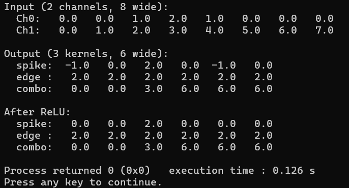
Figure 8-9 sends two input channels through three kernels and prints the result before and after ReLU. The spike kernel only has nonzero weights on channel 0, so it ignores the ramp on channel 1 entirely. Its output matches what we saw back in 044_1D_Convolution.c, a peak of 2.0 where the spike is, with −1.0 at the edges where the signal is rising or falling on one side only. The edge kernel does the opposite, it only looks at channel 1 and detects the rising slope of the ramp. Since the ramp increases steadily, the edge kernel produces a constant 2.0 at every position. The combo kernel pulls from both channels, applying {1, 0, −1} to channel 0 and {0, 1, 0} to channel 1, so its output blends information from the spike and the ramp together into something neither kernel could produce alone.
This is the full convolution operation as it actually works inside a neural network. Each output kernel reads from all input channels, multiplies by its own set of weights across every channel, sums everything together, and adds a bias. The result is one feature map per output kernel. After the convolution, ReLU clips the negative values to zero. You can see this in the “After ReLU” section: the −1.0 in the spike row disappears and everything else stays the same. The combination of multi-channel convolution followed by a nonlinear activation is the fundamental building block that gets stacked dozens or hundreds of times in modern convolutional networks. Every layer takes in a set of feature maps, applies a bank of learned kernels across all of them, and produces a new set of feature maps for the next layer to work with.
8.9 Why Convolution Works
Convolution has three properties that make it powerful for signals and images.
Weight sharing. The same kernel is used at every position. A spike detector with 3 weights works across 1000 samples. An MLP would need 1000 separate sets of 3 weights to do the same thing. This dramatically reduces the number of parameters.
Translation invariance. A pattern is detected the same way regardless of where it appears. A spike at sample 10 and a spike at sample 500 produce the same response. The network does not need to re-learn the pattern for each position.
Local connectivity. Each output only depends on a small window of the input (the kernel size). This matches the structure of signals and images where nearby values are related and distant values are less relevant.
These properties are assumptions about the data. They work beautifully for signals, images, and audio. They do not work for data where position does not matter (like tabular data with independent columns). Use MLPs for that.
8.10 Key Takeaways
Convolution slides a small kernel across the input, computing a weighted sum at each position. It is a dot product repeated at every location.
The kernel size determines how many input values each output depends on. The stride determines how far the kernel jumps. Padding adds zeros to preserve the spatial dimension.
Multiple kernels detect multiple features. Each kernel produces one output channel (feature map).
Output length = (input_length + 2*padding - kernel_length) / stride + 1.
Multi-channel convolution sums over input channels. The kernel has shape [out_channels][in_channels][kernel_width].
Weight sharing makes convolution parameter-efficient. A 3x3 kernel has 9 weights regardless of input size. An equivalent MLP would have thousands.
After convolution, apply an activation function (typically ReLU). In Chapter 9 we add pooling and stack multiple layers to build a complete CNN.
8.11 Exercises
Write a kernel that detects falling edges (transition from high to low). Apply it to the signal [0, 0, 1, 2, 1, 0, 0, 0] and verify it fires at the right location.
Apply a 5-wide averaging kernel [0.2, 0.2, 0.2, 0.2, 0.2] to a noisy signal. Generate noise with rand(). How does the output compare to the original clean signal?
Implement 2D convolution with padding and stride. Apply a 3x3 horizontal edge detector to a 5x5 image with a horizontal line.
Count the parameters in a convolution layer with 3 input channels, 16 output channels, and kernel size 3. Compare to a fully connected layer taking the same input (3 channels * 8 width = 24 inputs) and producing 16 outputs.
Implement the backward pass for 1D convolution. The gradient with respect to the kernel is the convolution of the input with the upstream gradient. The gradient with respect to the input is the “full” convolution of the kernel with the upstream gradient (flipped).
Look at KANN’s 1D convolution (kautodiff.c, search for kad_op_conv1d). It handles both NCW and NWC layouts. Which layout does your 049_Convolutional_Layer.c use?