CNN Architecture
Pooling, feature maps, and building a complete CNN
9.1 What You Will Learn
In Chapter 8 we built convolution from scratch and saw how kernels detect local patterns in signals and images. A single convolution layer can find edges, spikes, and simple transitions, but that is not enough to recognize anything complex. Detecting that there is an edge at position 12 and a spike at position 30 is useful, but what you really want to know is whether those features appear together in a particular arrangement, and that requires building up from local patterns to larger structures.
In this chapter we add the remaining pieces that turn convolution into a complete convolutional neural network. Pooling compresses the feature maps by summarizing local regions, reducing the spatial dimensions so that deeper layers can see a wider view of the input without needing enormous kernels. Stacking multiple convolution layers lets the network build hierarchical features, where the first layer detects simple patterns and each subsequent layer combines those patterns into something more abstract. Finally, flattening takes the 2D or multi-channel output of the last convolution layer and reshapes it into a single vector that can feed into a fully connected layer for classification. By the end of this chapter, you will have a complete CNN that takes a raw 1D signal as input and produces a classification output, with every operation implemented in C so you can see exactly what happens at each stage.
9.2 The Architecture
A CNN is a pipeline. Data flows through three types of operations, repeated in sequence.
Convolution - detect local patterns (edges, spikes, textures)
Activation - add non-linearity (ReLU)
Pooling - downsample, keeping only the strongest signals
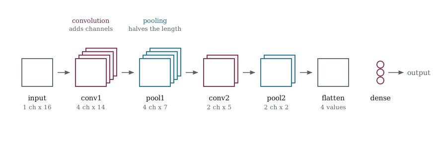
Figure 9-1 is the network assembled at the end of this chapter, drawn with the shapes it actually produces. A signal of 16 samples enters on the left, and by the time it reaches the dense layer it has become four numbers. Every stage in between either widens or shortens what passes through it, and reading the two numbers under each block from left to right tells you the whole story of a convolutional network.
Convolution adds channels without changing the length much, since one channel of 16 becomes four channels of 14, where each channel is the response of a different kernel to the same input. Pooling does the opposite and leaves the channel count alone while halving the length. Alternating the two means the representation gets deeper and shorter at the same time, until it is small enough that a handful of numbers describes the whole signal.
A CNN is a pipeline where data flows through the same sequence of operations repeated multiple times. First, a convolution layer scans the input with a bank of learned kernels to detect local patterns like edges, spikes, or textures. Second, an activation function like ReLU adds nonlinearity so the network can learn more than just linear combinations. Third, a pooling layer downsamples the feature maps by summarizing small regions into single values, keeping only the strongest responses and shrinking the spatial dimensions. After several rounds of convolution, activation, and pooling, the feature maps have gotten spatially smaller but richer in meaning. The first layer might detect simple edges, the second layer combines those edges into corners and curves, and by the third layer the network is responding to higher level structures built from all the layers below. Once the feature maps are small enough, we flatten them into a single 1D vector and feed that into a fully connected layer, which is the same kind of multilayer perceptron we built in Chapters 2 through 6. The dense layer takes the features that the convolutional layers extracted and uses them to make the final classification decision. A typical architecture looks like convolution, ReLU, convolution, ReLU, max pool, dropout, dense, ReLU, dense then softmax. Let us build each piece, you’re already familiar with convolution and activation so we’ll focus on pooling.
9.3 Max Pooling
Pooling reduces the spatial size of a feature map by summarizing small regions into single values. The most common form is max pooling, which slides a window across the feature map and keeps only the maximum value in each window, discarding everything else. Recall that a feature map is the output of a single kernel applied across the entire input. If a convolution layer has 8 kernels, it produces 8 feature maps, each one highlighting a different local pattern that its kernel learned to detect.
If a kernel in the previous layer detected an edge somewhere within a 2x2 region, max pooling does not care exactly which pixel triggered the strongest response. It just passes the strongest value forward and throws away the positional detail within that window. This does two things at once. It shrinks the feature map, which means fewer values for the next layer to process and fewer parameters needed downstream and it adds a small amount of translation invariance, because the exact position of a feature within each pooling window does not matter anymore. A spike that lands one pixel to the left or right still produces the same max pooled output, as long as it falls within the same window. The network becomes slightly less sensitive to small shifts in the input, which is usually what you want when you care about whether a pattern is present rather than precisely where it sits.
Let’s do this in C so you can properly see it in action.
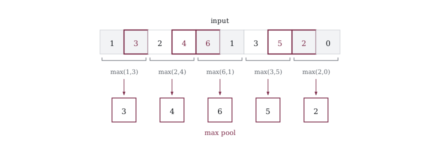
Figure 9-2 shows the rule applied to the ten samples the program uses. The input divides into five pairs, each pair is reduced to its larger value, and the survivors are highlighted in the input row so you can see which position won. Four of the ten values are discarded outright and never influence anything downstream.
That discarding is the point rather than a side effect. Whatever the convolution found, the strongest response in each neighborhood survives and its exact position within the pair does not, which is why a pooled feature map still reports that a pattern was present while becoming vague about precisely where. A spike one sample to the left produces the same pooled output.
/* 050_Max_Pooling.c */
#include <stdio.h>

/* 1D max pooling: take the max of each window of
   size pool_size */
static int maxpool1d(const float *input, int in_len,
                     int pool_size, int stride,
                     float *output, int *indices)
{
    int out_len = (in_len - pool_size) / stride + 1;
    int i, k;

    for (i = 0; i < out_len; i++) {
        int start = i * stride;
        float max_val = input[start];
        int max_idx = start;

        for (k = 1; k < pool_size; k++) {
            if (input[start + k] > max_val) {
                max_val = input[start + k];
                max_idx = start + k;
            }
        }
        output[i] = max_val;
        indices[i] = max_idx;
        /* save for backward pass */
    }
    return out_len;
}

int main(void)
{
    float input[] = { 1, 3, 2, 4, 6, 1, 3, 5, 2, 0 };
    int in_len = 10;
    float output[5];
    int indices[5];
    int out_len, i;

    /* Pool size 2, stride 2: halves the length */
    out_len = maxpool1d(input, in_len, 2, 2,
        output, indices);

    printf("Input (%d):  ", in_len);
    for (i = 0; i < in_len; i++)
        printf("%.0f ", input[i]);

    printf("\nPool 2x2 (%d): ", out_len);
    for (i = 0; i < out_len; i++)
        printf("%.0f ", output[i]);

    printf("\nMax index:    ");
    for (i = 0; i < out_len; i++)
        printf("%d ", indices[i]);

    printf("\n\n");

    /* Pool size 3, stride 3 */
    out_len = maxpool1d(input, in_len, 3, 3,
        output, indices);
    printf("Pool 3x3 (%d): ", out_len);
    for (i = 0; i < out_len; i++)
        printf("%.0f ", output[i]);
    printf("\n");

    return 0;
}
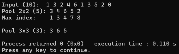
Figure 9-3 pools at window 2 and window 3 and reports the index each maximum came from. With pool size 2 and stride 2, the input gets split into consecutive pairs: {1,3}, {2,4}, {6,1}, {3,5}, {2,0}. From each pair the pooling layer keeps the larger value, giving the output {3, 4, 6, 5, 2}. Ten values become five. The max index row tells you exactly which position in the original input each output came from: the 3 came from index 1, the 4 came from index 3, the 6 came from index 4, and so on. Those indices matter because during backpropagation the gradient can only flow back to the element that actually produced the maximum. Every other element in the window had no effect on the output, so it gets zero gradient. The winning element receives the full gradient from above.
With pool size 3 and stride 3, the input gets split into groups of three: {1,3,2}, {4,6,1}, {3,5,2}. The maximum of each group gives {3, 6, 5}, and the last element in the input gets dropped because it does not fill a complete window. Ten values become three, a much more aggressive reduction. The larger the pool size, the more spatial detail gets thrown away in exchange for a smaller, more compact representation. Max pooling also gives the network a degree of translation invariance. If a feature shifts by one position within a pooling window, the maximum value in that window is likely the same, so the output does not change. The network becomes less sensitive to exactly where a pattern appears and more focused on whether it appears at all.
9.4 Average Pooling
Average pooling works the same way as max pooling structurally, sliding a window across the feature map and producing one value per window. The difference is that instead of keeping the largest value, it averages all the values in the window together. Every element in the window contributes equally to the output, so the result is a smoother, blurred version of the feature map rather than a selection of the strongest responses.
The tradeoff is straightforward. Max pooling is aggressive: it picks the single strongest activation and ignores everything else, which makes it good at preserving sharp features and edges. Average pooling is gentler: it considers the whole neighborhood, which means it retains more information about the overall level of activation in a region but can dilute a strong signal if it is surrounded by weak ones. A spike of 10 surrounded by four zeros comes through max pooling as 10, but through average pooling as 2. In practice, max pooling is more common in the early and middle layers of a CNN because those layers are trying to detect and preserve specific features. Average pooling shows up more often at the very end of a network, where the goal is to summarize an entire feature map into a single value before feeding it into the classifier.
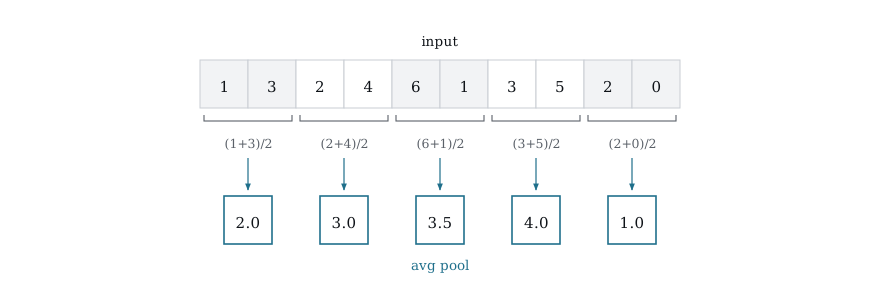
Figure 9-4 applies the other rule to the same input. Every value now contributes to its pair rather than competing with it, so nothing is discarded and nothing dominates. The third pair is the one to watch, where a 6 beside a 1 becomes 3.5 rather than 6.
/* 051_Average_Pooling.c */
#include <stdio.h>

static int avgpool1d(const float *input, int in_len,
                     int pool_size, int stride,
                     float *output)
{
    int out_len = (in_len - pool_size) / stride + 1;
    int i, k;

    for (i = 0; i < out_len; i++) {
        float sum = 0.0f;
        int start = i * stride;
        for (k = 0; k < pool_size; k++)
            sum += input[start + k];
        output[i] = sum / pool_size;
    }
    return out_len;
}

int main(void)
{
    float input[] = { 1, 3, 2, 4, 6, 1, 3, 5, 2, 0 };
    int in_len = 10;
    float max_out[5], avg_out[5];
    int i;

    /* Compare max vs average pooling */
    printf("Input:    ");
    for (i = 0; i < in_len; i++)
        printf("%.0f ", input[i]);

    /* Max pool */
    float tmp_out[5];
    int tmp_idx[5];
    int out_len = (in_len - 2) / 2 + 1;
    for (i = 0; i < out_len; i++) {
        int s = i * 2;
        max_out[i] = input[s] > input[s+1]
            ? input[s]
            : input[s+1];
    }
    printf("\nMax pool: ");
    for (i = 0; i < out_len; i++)
        printf("%.0f ", max_out[i]);

    /* Avg pool */
    avgpool1d(input, in_len, 2, 2, avg_out);
    printf("\nAvg pool: ");
    for (i = 0; i < out_len; i++)
        printf("%.1f ", avg_out[i]);

    printf("\n\nMax pool keeps the peaks. Avg pool "
           "smooths everything.\n");
    printf("Max pool is the default for "
           "classification.\n");
    printf("Avg pool is sometimes used as the final "
           "pooling before\n");
    printf("the classifier "
           "(global average pooling).\n");

    return 0;
}
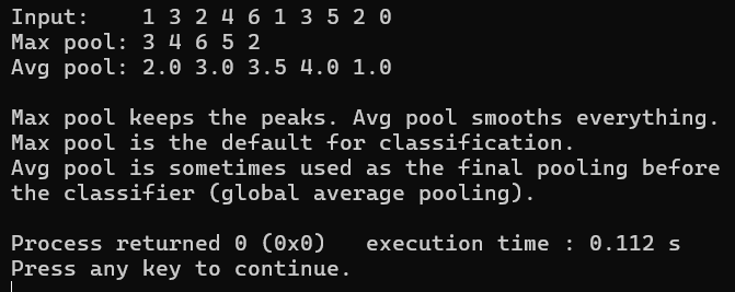
Figure 9-5 reduces the same five pairs by maximum and by average. The same input produces noticeably different results depending on which pooling method you use. The first pair {1, 3} gives 3 from max pooling but 2.0 from average pooling. The fourth pair {3, 5} gives 5 versus 4.0. Max pooling preserves the peaks and throws away the weaker value, while average pooling splits the difference and gives you something in between. If there is a strong activation in a feature map surrounded by weak ones, max pooling passes it through at full strength. Average pooling dilutes it.
For the intermediate layers of a CNN, max pooling is the standard choice because those layers are trying to detect whether specific features are present, and keeping the strongest response is more useful than averaging it with its neighbors. At the very end of a network, you sometimes see global average pooling, which takes an entire feature map and averages every value in it down to a single number. If the last convolution layer produces 64 feature maps, global average pooling gives you a vector of 64 values, one per channel, which feeds directly into the classifier. This avoids the large number of parameters that come with flattening a full feature map into a dense layer, and it works well when the network has learned feature maps where the overall level of activation matters more than the exact spatial location.
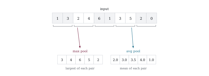
Figure 9-6 runs both pooling rules over the same ten samples, using the numbers the two programs print. The input is divided into five pairs, and each rule turns a pair into one number. Max pooling reports the larger of the two and average pooling reports their mean, which is the entire difference between them.
Look at the third pair, where 6 and 1 sit next to each other. Max pooling reports 6 and keeps the spike intact, while average pooling reports 3.5 and has halved it. That is the reason max pooling is the default after a convolution, because a convolution output is a record of where a pattern matched, and averaging a strong match against its quiet neighbor throws away the very thing the kernel was looking for.
9.5 Stacking Layers
A single convolution layer detects simple local features like edges and spikes. When you stack a second convolution layer on top, its kernels operate on the feature maps produced by the first layer rather than on the raw input. That means the second layer is detecting combinations of the simple features that the first layer found. A first layer neuron might respond to a horizontal edge, and a second layer neuron that combines several first layer outputs might respond to a corner, which is just two edges meeting at a specific angle. Add a third layer and you get combinations of combinations, patterns built from corners and curves that start to look like parts of objects.
This hierarchical feature detection is what makes CNNs so effective compared to a flat network that tries to learn everything in one shot. Each layer operates at a different level of abstraction, and the pooling between layers shrinks the spatial dimensions so that deeper layers can see a wider region of the original input through a smaller number of values. Let us stack two convolution layers with pooling in between and watch how the feature maps change from one layer to the next.
/* 052_Stacking_Conv.c */
#include <stdio.h>
#include <math.h>

static float relu(float z)
{
    return z > 0 ? z : 0;
}

/* Simplified conv1d: single input channel, single
   output channel */
static void conv1d_simple(const float *in, int in_len,
                           const float *ker,
                               int ker_len,
                           float bias, float *out,
                               int *out_len)
{
    *out_len = in_len - ker_len + 1;
    int i, k;
    for (i = 0; i < *out_len; i++) {
        float sum = bias;
        for (k = 0; k < ker_len; k++)
            sum += in[i + k] * ker[k];
        out[i] = relu(sum);
    }
}

static void maxpool(const float *in, int in_len,
                    float *out, int *out_len)
{
    *out_len = in_len / 2;
    int i;
    for (i = 0; i < *out_len; i++) {
        float a = in[i * 2], b = in[i * 2 + 1];
        out[i] = a > b ? a : b;
    }
}

int main(void)
{
    /* Input signal: two spikes */
    float input[16] = { 0, 0, 1, 3, 1, 0,
        0, 0, 0, 0, 0,
        1, 3, 1, 0, 0 };

    /* Layer 1: spike detector */
    float ker1[] = { -1, 2, -1 };
    float l1_out[16];
    int l1_len;
    conv1d_simple(input, 16, ker1, 3, 0,
        l1_out, &l1_len);

    /* Pool 1 */
    float p1_out[16];
    int p1_len;
    maxpool(l1_out, l1_len, p1_out, &p1_len);

    /* Layer 2: detects patterns in the pooled spike
       map */
    float ker2[] = { 1, -1, 1 };
    float l2_out[16];
    int l2_len;
    conv1d_simple(p1_out, p1_len, ker2, 3, 0,
        l2_out, &l2_len);

    int i;
    printf("Input (%d):         ", 16);
    for (i = 0; i < 16; i++) printf("%.0f ", input[i]);

    printf("\nConv1+ReLU (%d):     ", l1_len);
    for (i = 0; i < l1_len; i++)
        printf("%.0f ", l1_out[i]);

    printf("\nMaxPool (%d):         ", p1_len);
    for (i = 0; i < p1_len; i++)
        printf("%.0f ", p1_out[i]);

    printf("\nConv2+ReLU (%d):      ", l2_len);
    for (i = 0; i < l2_len; i++)
        printf("%.0f ", l2_out[i]);

    printf("\n\nThe input had 16 values. After two "
           "conv+pool stages\n");
    printf("we are down to %d values. Each value "
           "summarizes a\n", l2_len);
    printf("larger region of the original input.\n");

    return 0;
}
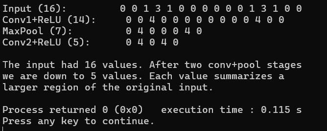
Figure 9-7 follows the signal through convolution, pooling and convolution again, and it shrinks at each stage. The input starts at 16 values, the first convolution with a kernel of 3 brings it down to 14, max pooling halves that to 7, and the second convolution reduces it further to 5. By the end, 16 values have been compressed into 5, and each of those 5 values carries information about a much larger region of the original signal than any single convolution could see on its own.
The first convolution layer looks at 3 consecutive samples at a time, so each output value is influenced by a window of 3 in the original input. After pooling, each value in the pooled output represents the stronger of two neighboring first layer outputs, so it effectively covers 4 samples of the original input. When the second convolution layer applies a kernel of width 3 to the pooled feature map, each of its output values draws from 3 pooled values, each of which already covers 4 original samples. That means a single output of the second layer is influenced by roughly 8 samples of the original input. This is called the receptive field, and it grows with every layer you add. The deeper you go in the network, the wider the region of the original input that each neuron can see, which is how the network builds up from detecting small local features to recognizing large scale patterns.
9.6 Flattening
After the convolution and pooling stages, the data sits in a multi-channel format where each channel is a feature map with a reduced spatial size. If the last pooling layer produces 8 channels each with 4 values, you have 8 separate arrays of 4 numbers. A fully connected layer expects a single flat vector as input, not a stack of separate feature maps, so we need to reshape the data before it can feed into the classifier.
Flattening does exactly what it sounds like. It takes all the feature maps and lays them end to end into one long 1D array. Those 8 channels of 4 values become a single vector of 32 values. No computation happens during flattening, no weights, no activation functions. It is purely a reshaping operation that takes the spatial, multi-channel output of the convolutional pipeline and arranges it into the format that a dense layer can work with. From that point on, the network is just a regular multilayer perceptron like the ones we built in the early chapters, taking a fixed length vector and producing class scores at the output.
/* 053_Flatten.c */
#include <stdio.h>

int main(void)
{
    /* Simulated output of conv layers: 4 channels, 3
       values each */
    float feature_maps[4][3] = {
        { 2.1f, 0.0f, 1.5f },
        { 0.0f, 3.2f, 0.0f },
        { 1.1f, 1.1f, 0.0f },
        { 0.0f, 0.0f, 2.8f },
    };
    int n_channels = 4, spatial_size = 3;

    /* Flatten: just read all values in order */
    int flat_size = n_channels * spatial_size;
    float flat[12];
    int c, s, idx = 0;

    for (c = 0; c < n_channels; c++)
        for (s = 0; s < spatial_size; s++)
            flat[idx++] = feature_maps[c][s];

    printf("Feature maps (4 channels x 3 spatial):\n");
    for (c = 0; c < n_channels; c++) {
        printf("  Ch%d: ", c);
        for (s = 0; s < spatial_size; s++)
            printf("%.1f ", feature_maps[c][s]);
        printf("\n");
    }

    printf("\nFlattened (%d values):\n  ", flat_size);
    for (idx = 0; idx < flat_size; idx++)
        printf("%.1f ", flat[idx]);
    printf("\n");

    printf("\nThis vector feeds into a dense layer for "
           "classification.\n");

    return 0;
}
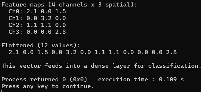
Figure 9-8 reads four feature maps out into one flat vector. Flattening has no weights and learns nothing. It simply takes the two-dimensional structure of channels and spatial positions and reads every value out in order into a single flat vector. Once the data is flattened, the dense layer that follows has no idea which values came from which channel or which spatial position. That information is gone from the structure of the data. But that is fine, because the whole point of the convolution and pooling layers before it was to encode the relevant spatial relationships into the values themselves. By the time the data reaches the flatten step, the important patterns have already been detected, combined, and compressed into the feature map values. The dense layer just needs to look at those values and decide which class they point to.
9.7 A Complete CNN
Let us put the full pipeline together. The input signal passes through a convolution layer that detects local features, followed by ReLU to add nonlinearity, followed by max pooling to downsample. That sequence repeats with a second convolution and pooling stage that detects higher level patterns in the compressed feature maps. After the second pooling, the feature maps get flattened into a single vector and fed into a dense layer, which is just a standard fully connected layer with weights and biases like the ones we built in the early chapters. The dense layer produces raw scores for each class, and softmax converts those scores into probabilities. We will build a 1D CNN that classifies simple signal patterns, with every stage implemented from scratch so you can trace the data from the raw input all the way through to the final class prediction.
/* 054_Complete_CNN.c */
#include <stdio.h>
#include <stdlib.h>
#include <math.h>
#include <float.h>

static float relu(float z)
{
    return z > 0 ? z : 0;
}

/* --- Convolution layer --- */
static void conv1d(const float *in,
    int in_ch, int in_w,
                   const float *ker, const float *bias,
                   int out_ch, int ker_w,
                   float *out, int *out_w)
{
    *out_w = in_w - ker_w + 1;
    int oc, ic, ow, kw;
    for (oc = 0; oc < out_ch; oc++) {
        for (ow = 0; ow < *out_w; ow++) {
            float sum = bias[oc];
            for (ic = 0; ic < in_ch; ic++)
                for (kw = 0; kw < ker_w; kw++)
                    sum += in[ic * in_w + ow + kw]
                      * ker[(oc * in_ch + ic)
                              * ker_w + kw];
            out[oc * (*out_w) + ow] = relu(sum);
        }
    }
}

/* --- Max pooling --- */
static void maxpool(const float *in,
    int channels, int in_w,
                    float *out, int *out_w)
{
    *out_w = in_w / 2;
    int c, i;
    for (c = 0; c < channels; c++) {
        for (i = 0; i < *out_w; i++) {
            float a = in[c * in_w + i * 2];
            float b = in[c * in_w + i * 2 + 1];
            out[c * (*out_w) + i] = a > b ? a : b;
        }
    }
}

/* --- Dense layer --- */
static void dense(const float *in, int in_size,
                  const float *w, const float *bias,
                  int out_size, float *out)
{
    int i, j;
    for (i = 0; i < out_size; i++) {
        float sum = bias[i];
        for (j = 0; j < in_size; j++)
            sum += w[i * in_size + j] * in[j];
        out[i] = sum;
    }
}

/* --- Softmax --- */
static void softmax(float *x, int n)
{
    float max_val = -FLT_MAX, sum = 0;
    int i;
    for (i = 0; i < n; i++)
        if (x[i] > max_val) max_val = x[i];
    for (i = 0; i < n; i++) {
        x[i] = expf(x[i] - max_val);
        sum += x[i];
    }
    for (i = 0; i < n; i++)
        x[i] /= sum;
}

int main(void)
{
    /* Three signal classes:
       0 = spike at start
       1 = spike in middle
       2 = spike at end */
    float signals[3][16] = {
        { 3, 1, 0, 0, 0, 0, 0, 0, 0, 0, 0, 0,
            0, 0, 0, 0 },
        { 0, 0, 0, 0, 0, 0, 0, 3, 1, 0, 0, 0,
            0, 0, 0, 0 },
        { 0, 0, 0, 0, 0, 0, 0, 0, 0, 0, 0, 0,
            0, 0, 1, 3 },
    };

    /* Hand-designed weights to demonstrate the
       architecture */

    /* Conv1: 1 input channel, 4 output channels,
       kernel size 3 */
    float conv1_w[4 * 1 * 3] = {
        2, -1, 0,    /* detects rising edge */
        0, -1, 2,    /* detects falling edge */
        -1, 2, -1,   /* detects spike */
        1, 1, 1,     /* smoother */
    };
    float conv1_b[4] = { 0, 0, 0, 0 };

    /* Conv2: 4 input channels, 2 output channels,
       kernel size 3 */
    float conv2_w[2 * 4 * 3];
    float conv2_b[2] = { 0, 0 };

    /* Initialize conv2 with small values */
    srand(42);
    int i;
    for (i = 0; i < 2 * 4 * 3; i++)
        conv2_w[i] = ((float)rand() / RAND_MAX)
            * 0.4f - 0.2f;

    /* Dense: flat_size -> 3 classes */
    /* We will compute flat_size after running the
       conv layers */

    float buf1[256], buf2[256], buf3[256];
    int w1, w2, w3;
    int s;

    /* Run each signal through the CNN */
    for (s = 0; s < 3; s++) {
        printf("Signal %d (spike at %s):\n", s,
              s == 0 ? "start"
                     : s == 1 ? "middle" : "end");

        /* Conv1: 1ch x 16 -> 4ch x 14 */
        conv1d(signals[s], 1, 16, conv1_w, conv1_b, 4,
            3, buf1, &w1);
        printf("  After conv1 (%d ch x %d): ", 4, w1);
        /* Just show channel 2 (spike detector) */
        printf("ch2=[");
        for (i = 0; i < w1; i++)
            printf("%.0f%s", buf1[2*w1+i],
                i<w1-1?",":" ");
        printf("]\n");

        /* Pool1: 4ch x 14 -> 4ch x 7 */
        maxpool(buf1, 4, w1, buf2, &w2);
        printf("  After pool1 (%d ch x %d): ", 4, w2);
        printf("ch2=[");
        for (i = 0; i < w2; i++)
            printf("%.0f%s", buf2[2*w2+i],
                i<w2-1?",":" ");
        printf("]\n");

        /* Conv2: 4ch x 7 -> 2ch x 5 */
        conv1d(buf2, 4, w2, conv2_w, conv2_b, 2,
            3, buf3, &w3);
        printf("  After conv2 (%d ch x %d)\n", 2, w3);

        /* Pool2: 2ch x 5 -> 2ch x 2 (drop last) */
        int w4 = w3 / 2;
        float buf4[256];
        maxpool(buf3, 2,
            w3 - (w3 % 2 ? 1 : 0), buf4, &w4);
        printf("  After pool2 (%d ch x %d)\n", 2, w4);

        /* Flatten */
        int flat_size = 2 * w4;
        printf("  Flattened: %d values -> ["
               , flat_size);
        for (i = 0; i < flat_size; i++)
            printf("%.2f%s", buf4[i],
                i < flat_size-1 ? ", " : "");
        printf("]\n\n");
    }

    printf("In a trained CNN, the dense layer after "
           "flattening\n");
    printf("would classify based on these features.\n");
    printf("The conv layers have already extracted the "
           "relevant\n");
    printf("patterns. The dense layer just reads the "
           "summary.\n");

    return 0;
}
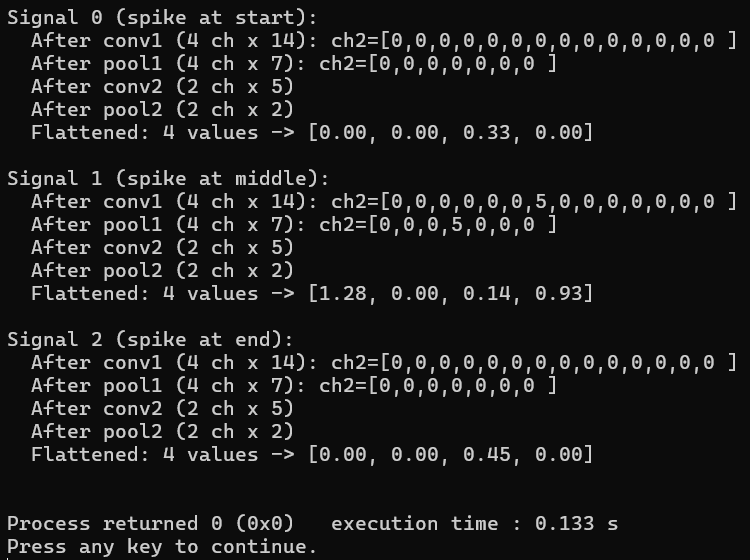
Figure 9-9 puts a complete CNN on the same spike at three positions. Follow the data through the pipeline and watch how it shrinks. The input starts at 16 values. The first convolution with a kernel of width 3 and no padding reduces it to 14. Max pooling with a window of 2 halves that to 7. The second convolution brings it down to 5, and the second pooling cuts it to 2. Two channels of 2 values each gives a flattened vector of just 4 numbers. The network has compressed a 16 sample signal down to 4 values, and those 4 values are what the classifier would use to decide which class the signal belongs to.
Look at channel 2, the spike detector, across the three signals. For signal 0, the spike is at the very start of the input, and the spike detector kernel {-1, 2, −1} does not fire because the spike pattern in this signal is {3, 1, 0}, a falling edge rather than a symmetric peak. For signal 1, the spike is in the middle and the detector fires strongly with a value of 5 at position 6. After pooling that 5 survives and ends up at position 3 in the pooled output. For signal 2, the spike is at the very end and the detector produces nothing because the pattern there is a rising edge {1, 3} at the boundary with no sample after it. Even though the spike detector does not fire for every signal, the other kernels, the rising edge detector, falling edge detector, and smoother, are all producing their own feature maps in parallel. The final flattened vectors are different for all three signals: {0.00, 0.00, 0.33, 0.00} versus {1.28, 0.00, 0.14, 0.93} versus {0.00, 0.00, 0.45, 0.00}. A dense layer looking at those vectors has enough information to tell the three classes apart, even though the spatial detail of where exactly the spike sat in the original 16 samples has been compressed away.
9.8 The Parameter Count Advantage
Let us count parameters to see why CNNs are so much more efficient than a fully connected network for spatial data.
Consider the signal we just processed: 16 input values, and we want to classify it into 3 classes. If you built a simple MLP with one hidden layer of 32 neurons, you would need 16 * 32 = 512 weights for the first layer plus 32 biases, then 32 * 3 = 96 weights for the output layer plus 3 biases. That is 643 parameters total, and every one of those connections treats the input as a flat bag of numbers with no spatial structure.
Now look at the CNN we just built. The first convolution layer has 4 kernels, each with 1 input channel and a width of 3, so that is 4 * 1 * 3 = 12 weights plus 4 biases. The second convolution layer has 2 kernels, each reading from 4 channels with a width of 3, so that is 2 * 4 * 3 = 24 weights plus 2 biases. The dense layer at the end takes a flattened vector of 4 values and maps to 3 classes, so that is 4 * 3 = 12 weights plus 3 biases. The total is 57 parameters. That is an order of magnitude fewer than the MLP, and the CNN is actually better at the task because it exploits the fact that the same pattern can appear at any position in the signal. The MLP has to independently learn “spike at position 0,” “spike at position 1,” “spike at position 2,” and so on. The CNN learns “spike” once and detects it everywhere.
/* 055_Parameter_Count.c */
#include <stdio.h>

int main(void)
{
    /* CNN for 1-channel, 16-wide input, 3 output
       classes */
    int conv1_params = 4 * 1 * 3 + 4;
    /* 4 filters, 1 in_ch, kernel 3, + bias */
    int conv2_params = 2 * 4 * 3 + 2;
    /* 2 filters, 4 in_ch, kernel 3, + bias */
    int flat_size = 2 * 2;
    /* 2 channels x 2 spatial after pooling */
    int dense_params = 3 * flat_size + 3;
    /* 3 classes */
    int cnn_total = conv1_params + conv2_params
        + dense_params;

    /* MLP for same input -> same output */
    int mlp_hidden = 32;
    int mlp_l1 = 16 * mlp_hidden + mlp_hidden;
    int mlp_l2 = mlp_hidden * 3 + 3;
    int mlp_total = mlp_l1 + mlp_l2;

    printf("CNN parameter count:\n");
    printf("  Conv1: %d filters x %d in_ch x %d kernel "
           "+ %d bias = %d\n",
           4, 1, 3, 4, conv1_params);
    printf("  Conv2: %d filters x %d in_ch x %d kernel "
           "+ %d bias = %d\n",
           2, 4, 3, 2, conv2_params);
    printf("  Dense: %d classes x %d flat + %d bias = "
           "%d\n",
           3, flat_size, 3, dense_params);
    printf("  Total: %d\n\n", cnn_total);

    printf("Equivalent MLP parameter count:\n");
    printf("  Layer 1: %d inputs x %d hidden + %d bias "
           "= %d\n",
           16, mlp_hidden, mlp_hidden, mlp_l1);
    printf("  Layer 2: %d hidden x %d classes + %d "
           "bias = %d\n",
           mlp_hidden, 3, 3, mlp_l2);
    printf("  Total: %d\n\n", mlp_total);

    printf("CNN uses %.1fx fewer parameters.\n",
           (float)mlp_total / cnn_total);
    printf("And the CNN would work on inputs of ANY "
           "length,\n");
    printf("not just 16. The MLP is fixed to 16 "
           "inputs.\n");

    return 0;
}
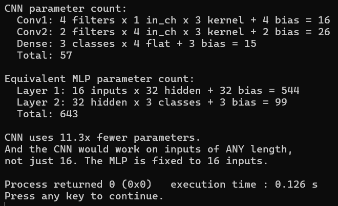
Figure 9-10 counts CNN parameters against the equivalent MLP, layer by layer. The CNN uses dramatically fewer parameters and generalizes across positions. An MLP trained on spikes at position 5 has to separately learn about spikes at position 10. A CNN learns “spike” once and detects it everywhere.
9.9 Key Takeaways
A CNN is a pipeline. conv -> relu -> pool, repeated, then flatten -> dense -> softmax.
Max pooling takes the maximum value in each window. It reduces spatial size, adds translation invariance, and keeps the strongest activations. The backward pass routes gradients only to the max positions.
Stacking conv+pool layers builds a hierarchy of features. Early layers detect simple patterns. Later layers detect combinations. Each layer’s receptive field covers a larger region of the original input.
Flattening reshapes the 2D feature maps (channels x spatial) into a 1D vector for the dense classifier. No parameters, just a reshape.
CNNs have far fewer parameters than equivalent MLPs because of weight sharing. A kernel works at every position, so it is learned once instead of once per position.
The architecture in KANN’s MNIST example (conv -> conv -> maxpool -> dropout -> dense -> softmax) is the pattern you will see in most practical CNNs, just with more layers and larger feature maps.
9.10 Exercises
Implement 2D max pooling with a 2x2 window and stride 2 on a 4x4 feature map. Verify the output is 2x2 with the correct maximum values.
Build a 2D CNN for a tiny image classification problem: create four 8x8 “images” (arrays) with different patterns (horizontal line, vertical line, diagonal, blank). Run them through conv2d -> relu -> maxpool -> flatten and compare the flattened vectors.
Compute the receptive field of the second convolution layer in 054_Complete_CNN.c. How many original input samples does each output value depend on?
Replace max pooling with average pooling in 054_Complete_CNN.c. Does it change the results? Why might max pooling work better for classification?
Add a third conv+pool stage to 054_Complete_CNN.c. What is the spatial size after the third pooling? What happens if the spatial size reaches 1?
Count the parameters in KANN’s MNIST CNN (32 filters, 3x3 kernel, two conv layers, 128-unit dense layer, 10 output classes). Compare to a fully connected network taking 784 inputs (28x28) to 128 hidden to 10 output.