Embeddings
Turning categories into learned vectors
10.1 What You Will Learn
So far our networks take numbers as input, sensor readings, pixel values, signal samples. But what if the input is a category? A word, a character, a product ID, a part number. You cannot multiply “hello” by a weight. You need a way to convert discrete categories into continuous vectors that the network can process. That is what embeddings do. In this chapter we build an embedding layer from scratch and see why it is one of the most important ideas in modern deep learning.
10.2 The Problem
Imagine you have 5 different sensor types and you want to include the sensor type as an input to your network. The obvious approach is to assign a number to each one: type 0, type 1, type 2, type 3, type 4. But the moment you do that, you have introduced a false ordering into the data. The network sees numbers and treats them like numbers, which means it thinks type 4 is somehow “more” than type 1, or that type 2 is halfway between type 1 and type 3. None of that is true. A thermocouple is not halfway between an accelerometer and a pressure sensor. These are categories, not quantities, and encoding them as a single number forces a relationship onto them that does not exist.
One-hot encoding fixes the ordering problem by giving each type its own binary column, so type 2 becomes {0, 0, 1, 0, 0}. But that creates a different problem. With 5 types you need 5 inputs, which is manageable. With 10,000 types you need 10,000 inputs, and almost all of them are zero for any given sample. The vectors are enormous and completely sparse, which wastes memory and gives the network nothing useful to work with because every type is equally distant from every other type. A thermocouple is just as far from a thermistor as it is from a gyroscope, even though the first two measure the same physical quantity. One-hot encoding cannot capture that kind of similarity.
10.3 One-Hot Encoding
The simplest fix is one-hot encoding. Represent each category as a vector of all zeros with a single 1 at the position corresponding to the category.
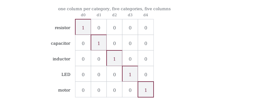
Figure 10-1 lays out what that produces for the five categories the first program uses. Each row is one category and each column is one input to the network, so the table is square by construction and grows in both directions as categories are added. Nothing in the arrangement says a resistor is nearer a capacitor than it is to a motor, which is the ordering problem solved, and every pair of rows sits exactly the same distance apart.
That even spacing is the cost as well as the benefit. The encoding refuses to claim a relationship that does not exist, and it also refuses to represent one that does.
/* 056_One_Hot_Encoding.c */
#include <stdio.h>
#include <string.h>

static void one_hot(int category,
    int n_categories, float *out)
{
    int i;
    for (i = 0; i < n_categories; i++)
        out[i] = 0.0f;
    out[category] = 1.0f;
}

int main(void)
{
    int n_categories = 5;
    float vec[5];
    int i, c;

    printf("One-hot encoding for 5 categories:\n\n");
    for (c = 0; c < n_categories; c++) {
        one_hot(c, n_categories, vec);
        printf("  Category %d: [", c);
        for (i = 0; i < n_categories; i++)
            printf("%.0f%s", vec[i],
                i < n_categories - 1 ? ", " : "");
        printf("]\n");
    }

    printf("\nNo ordering implied. Each category is "
           "equidistant\n");
    printf("from every other category (distance = "
           "sqrt(2)).\n");

    return 0;
}
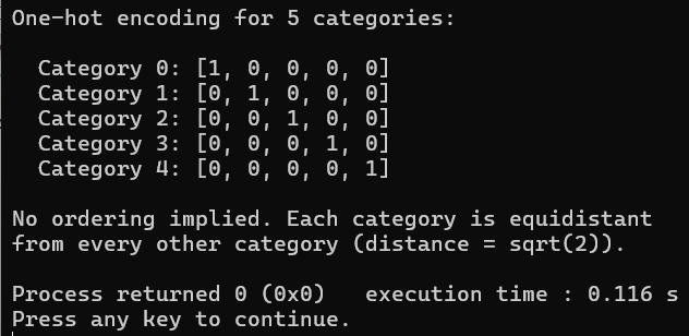
Figure 10-2 encodes five categories and leaves every pair the same distance apart. One hot encoding solves the ordering problem because every category gets its own dimension and no category is closer to or further from any other. The distance between any two one-hot vectors is always sqrt(2), regardless of what they represent. But the approach falls apart at scale. If your vocabulary has 50,000 words, every single word is represented as a vector of 50,000 floats with exactly one of them set to 1.0 and the rest all zero. That is 200KB per word just to say which word it is, and most of that memory is storing zeros.
The deeper problem is that one-hot encoding treats every category as equally unrelated to every other category. In one-hot space, “dog” is exactly as different from “cat” as it is from “refrigerator.” There is no way to express the idea that dogs and cats are both animals, or that “running” and “sprinting” mean nearly the same thing. Every word is an isolated point in a 50,000 dimensional space with no neighbors and no structure. What we really want is a representation where similar things are close together and dissimilar things are far apart, and where that similarity is learned from data rather than assigned by hand.
10.4 One-Hot Times a Weight Matrix
When you feed a one-hot vector into a dense layer, the math simplifies in a useful way. A dense layer computes output = W * input + bias, which normally means multiplying every weight by every input and summing across the full input dimension. But when the input is a one-hot vector, all the inputs are zero except for one position, say position k. Every weight that gets multiplied by zero contributes nothing to the sum. The only weights that matter are the ones connected to position k, which is just row k of the weight matrix.
So, the entire matrix multiplication collapses into a single row lookup. You do not need to do any multiplication at all. You just go to row k of the weight matrix and copy those values out. If the weight matrix has 50,000 rows and 64 columns, feeding in a one-hot vector for word 317 gives you the same result as just reading row 317, which is 64 values instead of 50,000. That is the key insight behind embeddings. Instead of storing the full one-hot vector and doing a wasteful matrix multiply where almost every term is zero, you skip the one-hot representation entirely and just store the weight matrix as a lookup table. Given a category index, you look up its row, and that row is the embedding vector for that category.
/* 057_Dense_One_Hot.c */
#include <stdio.h>

/* Dense layer: output[i] = sum(W[i][j] * input[j]) +
   bias[i] */
static void dense(const float *W, const float *bias,
                  const float *input, float *output,
                  int out_size, int in_size)
{
    int i, j;
    for (i = 0; i < out_size; i++) {
        float sum = bias[i];
        for (j = 0; j < in_size; j++)
            sum += W[i * in_size + j] * input[j];
        output[i] = sum;
    }
}

int main(void)
{
    /* 5 categories, embedding dimension 3 */
    /* Weight matrix: 3 rows x 5 columns */
    float W[3 * 5] = {
        0.1f, 0.5f, -0.3f, 0.8f, -0.2f,   /* row 0 */
        0.4f, -0.1f, 0.6f, 0.2f, 0.7f,    /* row 1 */
        -0.5f, 0.3f, 0.1f, -0.4f, 0.9f,   /* row 2 */
    };
    float bias[3] = { 0, 0, 0 };

    /* One-hot for category 1 */
    float input[5] = { 0, 1, 0, 0, 0 };
    float output[3];
    int i;

    dense(W, bias, input, output, 3, 5);

    printf("Weight matrix (3x5):\n");
    for (i = 0; i < 3; i++)
        printf("  [%.1f, %.1f, %.1f, %.1f, %.1f]\n",
               W[i*5], W[i*5+1], W[i*5+2],
                   W[i*5+3], W[i*5+4]);

    printf("\nOne-hot input (category 1): [");
    for (i = 0; i < 5; i++)
        printf("%.0f%s", input[i], i<4?", ":"");
    printf("]\n");

    printf("\nDense output: [%.1f, %.1f, %.1f]\n",
           output[0], output[1], output[2]);

    printf("\nColumn 1 of W: [%.1f, %.1f, %.1f]\n",
           W[1], W[1+5], W[1+10]);

    return 0;
}
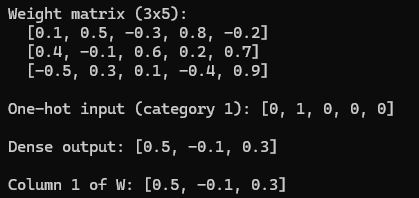
Figure 10-3 sends a one-hot vector through a dense layer. The output is {0.5, −0.1, 0.3}, which is exactly column 1 of the weight matrix. That is not a coincidence. When the input is a one-hot vector with a 1 at position 1, every column except column 1 gets multiplied by zero and contributes nothing. The entire dense layer computation, all 15 multiplications and 3 additions, produces the same result as just reading three values straight from the matrix.
An embedding layer takes this observation and makes it the whole design. Instead of constructing a one-hot vector, multiplying it through a weight matrix, and throwing away all the zero terms, you just store the weight matrix and index directly into it. Give it category 1, it returns row 1. Give it category 4, it returns row 4. No multiplication, no wasted memory on one-hot vectors, just a table lookup. The embedding matrix is still a learned parameter that gets updated during training through backpropagation, but the forward pass is a single array index instead of a matrix multiply.
10.5 The Embedding Layer
An embedding layer is just a lookup table stored as a 2D array of floats. You give it an integer index and it hands back the corresponding row from a weight matrix. There is no one-hot vector anywhere in the process, no matrix multiplication, no wasted computation. If you have 50,000 words and you want a 64-dimensional embedding for each one, the embedding layer is a 50,000 by 64 array. Word 317 maps to row 317, which gives you 64 floats. That is the entire forward pass for this layer.
The weight matrix is initialized with small random values, just like any other layer in the network. During training, backpropagation adjusts the rows so that categories which behave similarly in the training data end up with similar embedding vectors, and categories that behave differently end up far apart. The network discovers these relationships on its own. Nobody tells it that “dog” and “cat” should be close together. It learns that from seeing them appear in similar contexts during training. The result is a compact, dense representation where every element of the vector carries information, unlike the one-hot vector where 49,999 out of 50,000 elements are zero.
/* 058_Embedding_Layer.c */
#include <stdio.h>
#include <stdlib.h>

typedef struct {
    float *table;       /* [n_categories][embed_dim] */
    int n_categories;
    int embed_dim;
}
Embedding;

static Embedding embed_create(int n_categories,
    int embed_dim)
{
    Embedding e;
    int i;

    e.n_categories = n_categories;
    e.embed_dim = embed_dim;
    e.table = (float *)malloc(
        n_categories * embed_dim * sizeof(float));

    /* Initialize with small random values */
    for (i = 0; i < n_categories * embed_dim; i++)
        e.table[i] = ((float)rand() / RAND_MAX)
            * 0.2f - 0.1f;

    return e;
}

static const float *embed_lookup(const Embedding *e,
    int category)
{
    /* Just return a pointer to the right row */
    return &e->table[category * e->embed_dim];
}

static void embed_free(Embedding *e)
{
    free(e->table);
}

int main(void)
{
    Embedding e;
    int i, c;

    srand(42);
    e = embed_create(5, 3);
    /* 5 categories, 3-dimensional embeddings */

    printf("Embedding table (5 categories x 3 "
           "dimensions):\n\n");
    for (c = 0; c < 5; c++) {
        const float *vec = embed_lookup(&e, c);
        printf("  Category %d: [%+.3f, %+.3f, %+.3f]\n",
               c, vec[0], vec[1], vec[2]);
    }

    printf("\nLookup is O(1). No matrix multiply "
           "needed.\n");
    printf("The values are learned during training, "
           "just\n");
    printf("like any other weight in the network.\n");

    embed_free(&e);
    return 0;
}
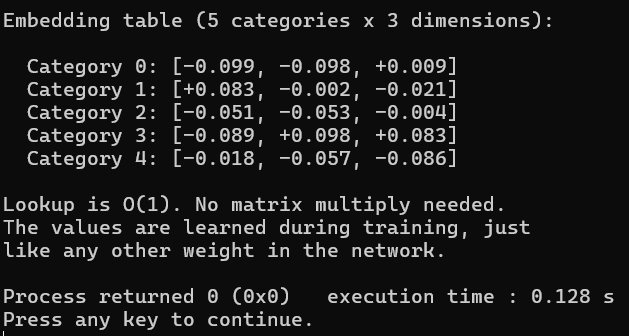
Figure 10-4 has the table and the lookup that replaces the matrix multiply. An embedding layer has n_categories * embed_dim learnable parameters. For a vocabulary of 50,000 words with 256 dimensions, that is 12.8 million parameters, which sounds enormous until you realize that a one-hot vector fed into a dense layer would require exactly the same number of parameters. The weight matrix is the same size either way because it has one row per category and one column per embedding dimension. The embedding layer does not save you any parameters. What it saves is computation and memory during the forward pass. The dense layer approach allocates a 50,000 element one-hot vector, multiplies 50,000 values by their corresponding weights for each output dimension, and throws away 49,999 zero terms. The embedding approach skips all of that and just copies 256 floats from the right row.
In practice, nobody actually builds a one-hot vector and multiplies it through a weight matrix. Every production system replaces that operation with a direct table lookup because the result is identical and the cost drops from O(n_categories * embed_dim) multiplications to O(embed_dim) memory copies. The math is equivalent, but the implementation is not, and at vocabulary sizes of tens or hundreds of thousands of words the difference in speed and memory usage is significant.
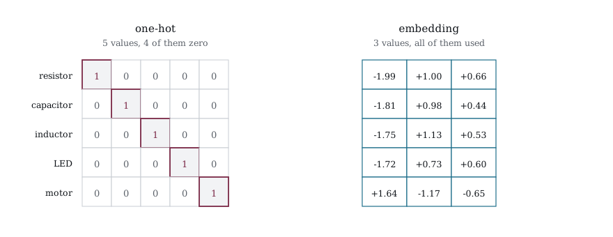
Figure 10-5 sets the two side by side for the same categories. On the left, five values per category of which four are always zero, so the width is fixed by how many categories exist. On the right, three values per category and every one of them carrying information, with the width chosen by us rather than dictated by the vocabulary. Add a thousand categories and the left side becomes a thousand columns wide while the right side stays at three.
10.6 What Embeddings Learn
The embedding vectors start out as random numbers with no meaning. During training, backpropagation pushes and pulls them the same way it adjusts any other weight in the network. Categories that appear in similar contexts get their vectors nudged in similar directions, and over many training steps they drift toward each other in embedding space. Categories that appear in different contexts get pushed apart. To make this concrete, imagine we have 6 categories representing electronic components: resistor, capacitor, inductor, LED, motor, and servo. We train a network on data about which parts are commonly used together in circuits. Resistors, capacitors, and inductors show up together in filter circuits, power supplies, and signal conditioning stages. Motors and servos show up together in actuator circuits and motor driver boards. LEDs sit somewhere in between, they appear in indicator circuits alongside resistors but not usually with motors.
After training, the embedding vectors should reflect these relationships. The three passive components should end up with similar vectors because they keep appearing in the same contexts. The two actuators should cluster together for the same reason. And the LED should land somewhere closer to the passives than to the actuators, because it shares more circuit context with a resistor than with a motor. Nobody tells the network any of this. It discovers the structure from the training data alone.
/* 059_Embeddings_Learn.c */
#include <stdio.h>
#include <stdlib.h>
#include <math.h>

static float randf(void)
{
    return (float)rand() / RAND_MAX;
}

/* Embedding + simple predictor: given two parts,
   predict
   if they appear in the same circuit (1) or not (0) */

#define N_PARTS 6
#define EMBED_DIM 3

static float sigmoid(float z)
{
    return 1.0f / (1.0f + expf(-z));
}

/* Predict similarity: dot product of embeddings ->
   sigmoid */
static float predict(
        const float embed[N_PARTS][EMBED_DIM],
                     int part_a, int part_b)
{
    float dot = 0;
    int i;
    for (i = 0; i < EMBED_DIM; i++)
        dot += embed[part_a][i] * embed[part_b][i];
    return sigmoid(dot);
}

int main(void)
{
    float embed[N_PARTS][EMBED_DIM];
    const char *names[] = { "resistor",
        "capacitor", "inductor",
                            "LED", "motor", "servo" };

    /* Training pairs: (part_a, part_b, co-occur?) */
    int pairs[][3] = {
        /* resistor + capacitor: yes (RC filter) */
        {0, 1, 1},
        /* resistor + inductor: yes (RL filter) */
        {0, 2, 1},
        /* capacitor + inductor: yes (LC tank) */
        {1, 2, 1},
        /* resistor + LED: yes (current limiting) */
        {0, 3, 1},
        {4, 5, 1},  /* motor + servo: yes (robotics) */
        {0, 4, 0},  /* resistor + motor: rarely */
        {1, 5, 0},  /* capacitor + servo: rarely */
        {2, 4, 0},  /* inductor + motor: rarely */
        {3, 5, 0},  /* LED + servo: rarely */
    };
    int n_pairs = 9;

    float lr = 0.5f;
    int epoch, p, i;

    srand(42);
    for (i = 0; i < N_PARTS * EMBED_DIM; i++)
        ((float*)embed)[i] = randf() * 0.4f - 0.2f;

    /* Train */
    for (epoch = 0; epoch < 500; epoch++) {
        for (p = 0; p < n_pairs; p++) {
            int a = pairs[p][0], b = pairs[p][1];
            float t = (float)pairs[p][2];
            float y = predict(embed, a, b);
            float err = y - t;

            /* Gradient: d_loss/d_embed[a][i] = err *
               y*(1-y) * embed[b][i]
                         d_loss/d_embed[b][i] = err * y
                             *(1-y) * embed[a][i] */
            float d = err * y * (1.0f - y);
            for (i = 0; i < EMBED_DIM; i++) {
                float ga = d * embed[b][i];
                float gb = d * embed[a][i];
                embed[a][i] -= lr * ga;
                embed[b][i] -= lr * gb;
            }
        }
    }

    /* Print learned embeddings */
    printf("Learned embeddings "
           "(%d-dimensional):\n\n", EMBED_DIM);
    for (i = 0; i < N_PARTS; i++)
        printf("  %-10s [%+.3f, %+.3f, %+.3f]\n",
               names[i], embed[i][0], embed[i][1],
                   embed[i][2]);

    /* Print distances */
    printf("\nDistances between parts:\n\n");
    int a, b;
    for (a = 0; a < N_PARTS; a++) {
        for (b = a + 1; b < N_PARTS; b++) {
            float dist = 0;
            for (i = 0; i < EMBED_DIM; i++) {
                float d = embed[a][i] - embed[b][i];
                dist += d * d;
            }
            dist = sqrtf(dist);
            printf("  %-10s <-> %-10s  dist=%.3f\n",
                   names[a], names[b], dist);
        }
    }

    return 0;
}
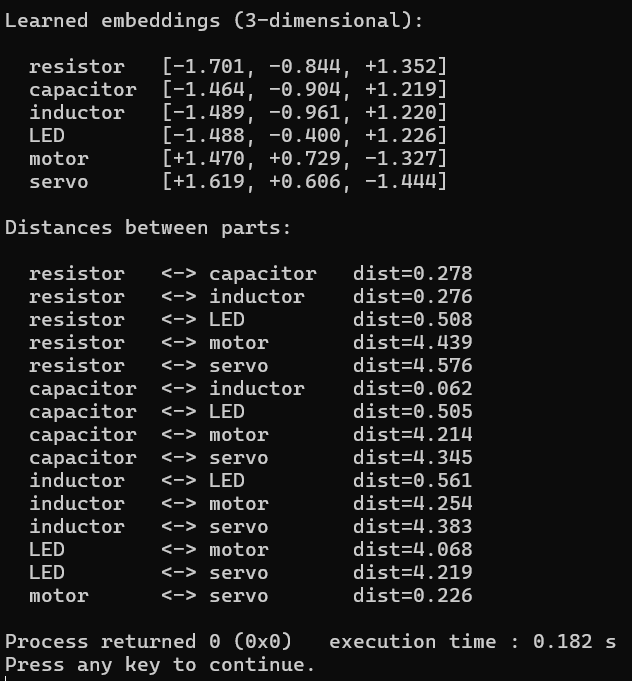
Figure 10-6 has the learned vectors for eight parts and the distances between them. Resistor, capacitor, and inductor should all be close to each other because they kept appearing together in the training pairs, they are the components you find side by side in filter circuits and power supplies. Motor and servo should also be close to each other because they co-occur in robotics and actuator circuits. But the distance between the passives group and the actuators group should be larger, because those parts rarely showed up together in the training data.
The network was never told that a resistor is a passive component or that a servo is an actuator. It does not know anything about electronics. All it saw was which parts appeared together and which did not, and from that co-occurrence information alone it arranged the embedding vectors so that related parts ended up nearby in 3D space. This is the same principle behind word embedding systems like Word2Vec and GloVe, which learn vector representations for words by looking at which words appear near each other in large bodies of text. Words that show up in similar contexts, like “king” and “queen” or “cat” and “dog,” end up with similar vectors because the training process pushes them together through the same gradient updates we just implemented. The embedding captures meaning not from any definition or label, but purely from patterns of usage.
10.7 The Backward Pass
During training, the gradient for an embedding layer only affects the row that was actually looked up. If the input was category 317, then row 317 gets updated and the other 49,999 rows stay exactly where they are. This is fundamentally different from a dense layer, where every weight participates in every forward pass and every weight gets a gradient on every backward pass.
This sparsity is what makes embedding layers practical at scale. If you have a vocabulary of 50,000 words and a batch of 32 training samples, only 32 rows get touched on each update. The vast majority of the embedding table sits idle on any given step. Over the course of training, every row eventually gets updated because every word appears somewhere in the dataset, but on each individual step the work is minimal. The gradient computation itself is simple: whatever gradient flows back from the layer above gets written directly into the gradient slot for that one row, with no summation across inputs because no other input contributed to the output.
Let us make this explicit by implementing the backward pass and watching which rows change and which stay frozen.
/* 060_Embeddings_Backward_Pass.c */
#include <stdio.h>
#include <stdlib.h>
#include <string.h>

#define N_CAT 5
#define EMBED_DIM 3

typedef struct {
    float table[N_CAT][EMBED_DIM];
    float grad[N_CAT][EMBED_DIM];
}
Embedding;

static void embed_zero_grad(Embedding *e)
{
    memset(e->grad, 0, sizeof(e->grad));
}

static const float
    *embed_forward(const Embedding *e, int cat)
{
    return e->table[cat];
}

static void embed_backward(Embedding *e, int cat,
                            const float *upstream_grad)
{
    /* Only the selected row gets gradient */
    int i;
    for (i = 0; i < EMBED_DIM; i++)
        e->grad[cat][i] += upstream_grad[i];
}

static void embed_update(Embedding *e, float lr)
{
    int i, j;
    for (i = 0; i < N_CAT; i++)
        for (j = 0; j < EMBED_DIM; j++)
            e->table[i][j] -= lr * e->grad[i][j];
}

int main(void)
{
    Embedding e;
    int i, j;

    /* Initialize */
    srand(42);
    for (i = 0; i < N_CAT; i++)
        for (j = 0; j < EMBED_DIM; j++)
            e.table[i][j] = ((float)rand() / RAND_MAX)
                * 0.2f - 0.1f;

    /* Simulate: look up category 2, get some
       upstream gradient */
    int cat = 2;
    embed_zero_grad(&e);

    printf("Before update (category %d):\n", cat);
    printf("  Embedding: [%.4f, %.4f, %.4f]\n",
           e.table[cat][0], e.table[cat][1],
               e.table[cat][2]);

    /* Pretend the upstream gradient is [0.1, -0.2,
       0.05] */
    float upstream[] = { 0.1f, -0.2f, 0.05f };
    embed_backward(&e, cat, upstream);

    printf("\n  Upstream gradient: "
           "[%.2f, %.2f, %.2f]\n",
           upstream[0], upstream[1], upstream[2]);
    printf("  Gradient buffer:\n");
    for (i = 0; i < N_CAT; i++) {
        printf("    Cat %d: [%.2f, %.2f, %.2f]", i,
               e.grad[i][0], e.grad[i][1],
                   e.grad[i][2]);
        if (i == cat)
            printf("  <-- only this row has gradient");
        printf("\n");
    }

    embed_update(&e, 0.1f);

    printf("\nAfter update:\n");
    printf("  Category %d: [%.4f, %.4f, %.4f]\n",
           cat, e.table[cat][0], e.table[cat][1],
               e.table[cat][2]);

    /* Show that other categories did not change */
    printf("  Category 0: [%.4f, %.4f, %.4f] "
           "(unchanged)\n",
           e.table[0][0], e.table[0][1], e.table[0][2]);

    return 0;
}
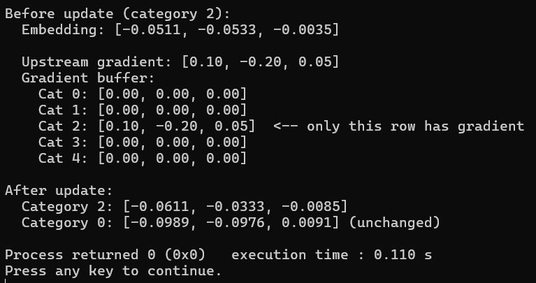
Figure 10-7 updates one embedding row and leaves the other four exactly where they were. Only category 2′s row changed. The other four rows came out of the update with exactly the same values they had before, because their gradients were all zeros. In this example with 5 categories the waste is small, but imagine a vocabulary of 50,000 words. Looping through all 50,000 rows and multiplying by zero 49,999 times would be absurd. Production systems avoid this by tracking which rows were accessed during the forward pass and only updating those rows during the backward pass. The embedding gradient is naturally sparse, only one row out of the entire table gets a nonzero gradient per input sample, and a good implementation takes advantage of that.
10.8 From Embeddings to Language
Embeddings are the bridge between discrete data and neural networks. A neural network operates on continuous numbers, it multiplies, adds, and applies activation functions to floats. But words, characters, and categories are not continuous. They are discrete symbols with no natural numerical representation. The embedding layer solves that problem by assigning each symbol a learned vector of floats, turning a discrete lookup into a continuous representation that the rest of the network can work with.
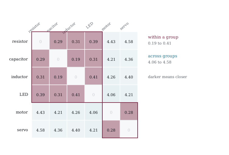
Figure 10-8 is every distance the program prints, arranged as a grid. Two blocks fall out of it without anyone drawing them, one covering the four passive parts and one covering the motor and the servo, and inside those blocks the distances run from 0.19 to 0.41 while every distance crossing between them runs from 4.06 to 4.58. The gap is a factor of ten and there is nothing in between.
Nothing told the network that a resistor and a capacitor belong together, and no two category labels were ever compared against each other during training. The grouping is a side effect of the task, because parts used the same way had to produce the same predictions, and the cheapest way to satisfy that was to give them nearby vectors. That is the property language models are built on. Nobody writes down what a word means, and the meaning arrives as geometry because words used alike end up placed alike.
In the next chapter we will build tokenization, which is the process of breaking text into small pieces and assigning each piece an integer ID. Each token ID gets looked up in an embedding table, and the result is a sequence of vectors, one per token, that captures the meaning of each piece as learned from training data. This sequence of vectors is what actually feeds into the network. Every language model follows this same pipeline: raw text goes in, the tokenizer breaks it into tokens, each token maps to an integer ID, the embedding layer converts each ID into a vector, and the neural network processes the resulting sequence of vectors to make its prediction. The embedding layer is the front door to every model we build from here on. RNNs, LSTMs, and transformers all operate on these learned vectors, never on raw text.
10.9 Key Takeaways
Categories cannot be used as raw numbers because the ordering is arbitrary. One-hot encoding solves this but wastes memory and computation.
Multiplying a one-hot vector by a weight matrix just selects one row. An embedding layer skips the multiplication and does a direct table lookup.
Embedding vectors are learned during training. Categories that appear in similar contexts end up with similar vectors. The network discovers relationships from data.
The backward pass only updates the row corresponding to the input category. The gradient is naturally sparse.
Embedding dimension is a hyperparameter. Common values: 32 to 512 for words, 8 to 64 for small categorical features. Larger dimensions capture more nuance but cost more memory.
Embeddings are the bridge between discrete data (words, tokens, part numbers) and continuous vector spaces that neural networks operate on.
10.10 Exercises
Compute the memory savings of an embedding lookup vs. one-hot + dense layer for 10,000 categories with 128-dimensional embeddings. Both store the same weight matrix, but what does the input representation cost?
Add a third dimension to the parts example (059_Embeddings_Learn.c) by including more parts (transistor, diode, relay) and more co-occurrence pairs. Do the clusters still form?
Implement an embedding layer where multiple categories are active at once (bag of words). Instead of looking up one row, sum the rows for all active categories. What does this represent?
Verify numerically that embed_forward on a one-hot vector through a dense layer produces the same result as embed_lookup. Use the same weight matrix for both.
What happens if the embedding dimension is 1? Each category is just a single number. Is this useful? When would it fail?
Implement cosine similarity between embedding vectors: cos(a,b) = dot(a,b) / (|a| * |b|). After training 059_Embeddings_Learn.c, which pairs have the highest cosine similarity?