LSTM
Gates that control what to remember and forget
15.1 What You Will Learn
Chapter 14 left the basic RNN in a bad place. Gradients travelling backward through time get multiplied by the tanh derivative and by W_h at every single step. After twenty or thirty steps there is nothing left of them to learn from. We measured a first step gradient roughly two hundred thousand times smaller than the last one over a thirty step sequence. No learning rate rescues a number that small and no amount of training time does either. The problem is built into the architecture rather than sitting in the code.
The Long Short-Term Memory network, published by Hochreiter and Schmidhuber in 1997, fixes it by changing the road the gradient travels on. Instead of forcing every signal through a squashing function and a matrix multiply once per step, the LSTM adds a second state vector called the cell state. That vector is connected from one step to the next by addition. Addition has a derivative of one, so gradient moving along the cell state loses nothing to the passage of time. That single structural change is the entire reason the architecture exists. Adding a clear channel raises an obvious question though, which is what decides what travels along it.
The answer is gates.
There are three of them, each a small sigmoid network producing a number between 0 and 1 that acts as a valve. One decides how much of the old memory survives, one decides how much new information gets written, and one decides how much of the memory is exposed to the rest of the network. The gates sit beside the channel rather than across it, which is what keeps the channel clear.
In this chapter we build the whole thing in C, one gate at a time, with every step compiling and running on its own. We start with the forget gate alone, then add the input gate and the candidate value it writes. Those combine into the cell state update, the output gate goes on after that, and and the complete cell comes together after that. The chapter finishes by running an LSTM and a basic RNN side by side on a sequence long enough to break the RNN, and then counts the parameter cost, because four times as many weights is not free and you should know what you are buying with it.
15.2 The Core Idea
The basic RNN asks one state vector to do three jobs at once, since h has to store what happened earlier, absorb whatever arrives now, and serve as the thing the output layer reads. Those jobs pull in different directions. Storage wants a value that survives untouched across many steps, while processing wants a value that changes in response to every input, and one vector cannot do both well. The LSTM stops asking and it splits the state into two vectors with different jobs.
The cell state c is long-term memory. Information travels along it with almost no transformation, which is what makes it the gradient highway named at the start of the chapter. Nothing squashes it and no matrix multiplies it as it moves from step to step. The hidden state h is short-term working memory. This is the vector the output layer sees, and it is derived from the cell state rather than being the cell state.
Controlling the traffic between them takes three gates, each of which is a small sigmoid network producing values between 0 and 1. A gate output of 0 closes the valve completely and a gate output of 1 opens it completely, and everything in between is a partial opening applied element by element. The forget gate f decides how much of the old cell state survives, where 0 erases and 1 keeps. The input gate i decides how much new information gets written into the cell state and the output gate o decides how much of the cell state is exposed as the hidden state.
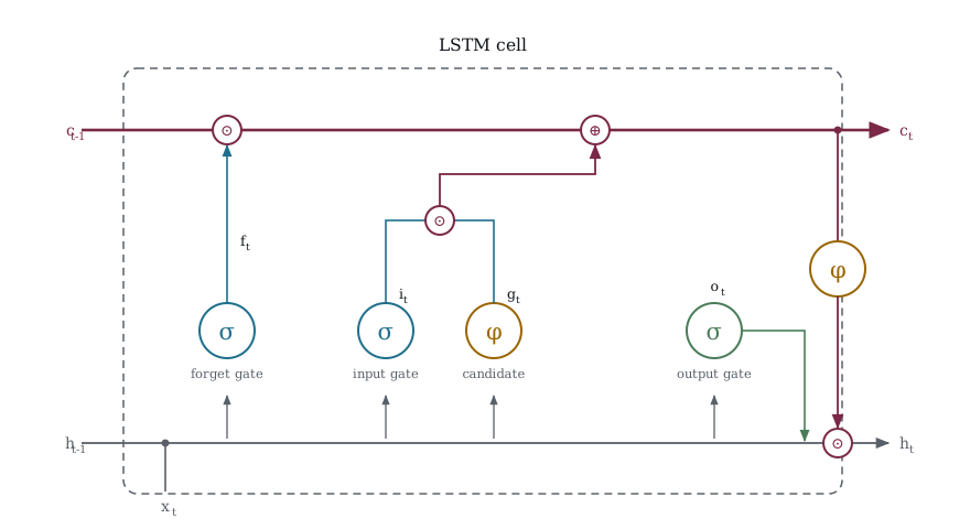
Figure 15-1 has the whole cell. Read the diagram along the top line first, because that line is the whole point of the architecture. The cell state enters on the left as c_{t-1} and leaves on the right as c_t, and between those two points it meets exactly two operations, a multiply and an add, both circled on the rail. It is never squashed and never multiplied by a weight matrix, which is why gradient survives the trip. Everything below that line is machinery deciding what those two operations do. Look at the bottom of the diagram and you will see that h_{t-1} and x_t both fan out to every box, so each gate sees the previous hidden state and the current input and makes its own decision from the pair.
One box needs explaining because it is not a gate. The diagram shows four boxes, f, i, g and o, but we have only named three gates. The odd one out is g, the candidate, and it uses tanh rather than sigmoid because its job is producing content rather than controlling a valve. The input gate i decides how much to write, and g is what gets written. We build those two together for exactly that reason.
Let us build each piece.
15.3 The Forget Gate
The forget gate decides what to throw away from the cell state. It looks at the current input and the previous hidden state, and outputs a number between 0 and 1 for each cell. A value of 1 means “keep everything.” A value of 0 means “erase completely.”
/* 081_Forget_Gate.c */
#include <stdio.h>
#include <math.h>

static float sigmoid(float z)
{
    return 1.0f / (1.0f + expf(-z));
}

#define N 3  /* cell size */

/* f = sigmoid(W_f * x + U_f * h_prev + b_f) */
static void forget_gate(float x,
                        const float W_f[N],
                        const float U_f[N][N],
                        const float b_f[N],
                        const float h_prev[N],
                        float f[N])
{
    int i, j;
    for (i = 0; i < N; i++) {
        float z = b_f[i] + W_f[i] * x;
        for (j = 0; j < N; j++)
            z += U_f[i][j] * h_prev[j];
        f[i] = sigmoid(z);
    }
}

/* A gate near 1 keeps, a gate near 0 erases, and
   anything between the two partly keeps */
static const char *label(float g)
{
    if (g > 0.8f) return "keep";
    if (g < 0.3f) return "erase";
    return "partial";
}

int main(void)
{
    /* Bias initialized to 1.0, as KANN does, so the
       gate starts open. The network begins by
       remembering everything and learns what to
       forget. */
    float W_f[N] = { -2.0f, 1.0f, 0.5f };
    float U_f[N][N] = {{ 0.1f, 0, 0 },
                       { 0, 0.1f, 0 },
                       { 0, 0, 0.1f }};
    /* initialized to 1 */
    float b_f[N] = { 1.0f, 1.0f, 1.0f };

    float h_prev[N] = { 0.5f, 0.3f, 0.8f };
    float inputs[] = { -2.0f, -1.0f, 0.0f,
                        0.5f, 1.0f, 1.5f };
    int n_inputs = 6;
    float f[N];
    int t, i;

    printf("Forget gate output for different "
           "inputs:\n\n");
    printf("  input   f[0]    f[1]    f[2]  ");
    printf("  cell 0   cell 1   cell 2\n");

    for (t = 0; t < n_inputs; t++) {
        forget_gate(inputs[t], W_f, U_f, b_f,
                    h_prev, f);
        printf("  %+4.1f    %.3f   %.3f   %.3f  ",
               inputs[t], f[0], f[1], f[2]);
        for (i = 0; i < N; i++)
            printf("  %-7s", label(f[i]));
        printf("\n");
    }

    printf("\nThe bias of 1.0 makes the gate start "
           "open (keep).\n");
    printf("This is important: KANN initializes the "
           "forget gate\n");
    printf("bias to 1.0 "
           "(see Jozefowicz et al, 2015).\n");
    printf("Without this, the LSTM forgets everything "
           "at startup\n");
    printf("and training is much harder.\n");

    return 0;
}
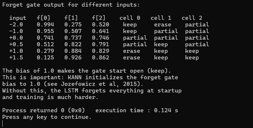
Figure 15-2 sweeps an input across the gate. Read the table down the rows and the first thing that should jump out is that the three cells almost never agree with each other. At an input of −2.0 the gate tells cell 0 to keep, with a value of 0.994, while at the same moment it tells cell 1 to erase at 0.275, and that is the same input arriving with the same previous hidden state producing two opposite instructions. Walk down to the bottom row at +1.5 and the pair have completely swapped places, cell 0 now sitting at 0.125 and cell 1 at 0.926. That disagreement is the entire reason the gate produces a vector rather than a single number, because if it were one number every memory in the cell would have to survive or die together and the cell state would collapse into a single accumulator instead of a set of independent slots the network can manage separately.
Why do they disagree? Look at W_f, which is set to −2.0, 1.0 and 0.5, so cell 0 responds strongly and negatively to whatever arrives, cell 1 responds positively, and cell 2 responds positively but so weakly that it barely moves across the whole sweep, drifting from 0.520 up to 0.862 while the bias does most of the work. In a real network you would never pick these by hand, they come out of training, and what the network is learning when it learns them is which inputs ought to clear which slots.
The middle row is the one to sit with though. At an input of 0.0 all three gates land at roughly 0.74, which is no coincidence at all, because with nothing arriving to react to each gate collapses to sigmoid of its own bias plus a small nudge from h_prev, and sigmoid(1.0) happens to be 0.7311. That is what the gate does before it knows anything, and the rest of this section is about why we chose that particular starting point rather than any other.
The forget gate uses sigmoid because it needs an output between 0 and 1 to behave like a switch at all, and this is exactly where sigmoid belongs in a recurrent network, not on the hidden state, which is tanh as we worked through in Chapter 13, but on the gates. Take that as a rule going forward since it holds for every architecture in the next four chapters. Sigmoid for anything that controls flow, tanh for anything that carries content.
It is worth asking what would happen if we reached for one of the other activations instead, because each one breaks the gate in its own specific way. Tanh runs from −1 to +1, and a negative multiplier applied to a stored memory does not reduce that memory at all, it flips its sign, which is a completely different operation and not one any gate has any business performing. ReLU fails at the other end since it is unbounded above, so a gate output of 3.0 would triple the cell state rather than preserving some fraction of it, and a cell state that gets tripled once per step is just the exploding gradient problem wearing a different hat. Sigmoid is the only one of the three that gives you a multiplier which can attenuate without ever inverting or amplifying, which is precisely the job description.
Now look at that bias initialization of 1.0, because that single constant matters far more than it appears to. KANN sets it explicitly with b = kann_new_vec(n1, 1.0f) and leaves a comment pointing at the Jozefowicz et al paper from 2015. Leave it at the usual 0 instead and the gate starts at sigmoid(0), which is exactly 0.5, meaning the cell state gets halved at every single step before the network has learned anything whatsoever about the task.
Follow that halving out for a few steps and the arithmetic should look uncomfortably familiar. Twenty steps of multiplying by 0.5 leaves you with 9.5e-07 of the original signal, fifty steps leaves 8.9e-16, and that last number sits in the same territory as the 3.76e-15 we measured for the plain RNN back in Chapter 14. So an LSTM initialized the ordinary way spends its early training fighting the exact failure the architecture was built to solve, and it has to climb out of that hole before it can even begin learning what you actually asked it to learn.
Starting the bias at 1.0 puts the gate at 0.7311 instead, and twenty steps of that leaves 0.0019, which is roughly two thousand times more signal surviving the same distance. I should be honest that this is still decay and not a perfect highway, since a freshly initialized LSTM does not preserve memory forever and nobody should claim otherwise. What the bias actually buys you is a network that starts out mostly remembering and then learns what to throw away, rather than one that starts out throwing everything away and has to learn how to hold on, and refining something that already half works is a far kinder optimization problem than repairing something broken.
That handles removal, but a gate that can only delete is not much use on its own. Something still has to decide what gets written into the cell in the first place, and that turns out to need two pieces working together rather than one.
15.4 The Input Gate and Candidate
The forget gate only ever removes, so something has to put information in. Writing turns out to involve two separate decisions rather than one, because the network has to settle both what the new value should be and how much of it actually belongs in the cell, and those are different questions with different answers. The LSTM answers them with two small networks running side by side off the same inputs. The candidate g uses tanh and produces the value that could be written, while the input gate i uses sigmoid and produces a fraction saying how much of that value gets through. Multiply them together and you have the new information, which is what the cell state update in the next section adds.
You might reasonably ask why the network needs both when a single tanh unit could just output a small number to mean write a little. The trouble is that magnitude and confidence would then be tangled together in one value, and the network would have no way of saying that a piece of information is large but uncertain. With the pair split apart, g can insist the content is +0.9 while i holds the valve at 0.1, and the two can be learned independently.
/* 082_Input_Gate.c */
#include <stdio.h>
#include <math.h>

static float sigmoid(float z)
{
    return 1.0f / (1.0f + expf(-z));
}
static float my_tanh(float z)
{
    if (z < -20) return -1;
    float e = expf(-2 * z);
    return (1 - e) / (1 + e);
}

#define N 3

int main(void)
{
    /* Input gate: i = sigmoid(W_i * x + U_i * h +
       b_i) */
    /* Candidate:  g = tanh(W_g * x + U_g * h + b_g) */

    float x = 1.0f;
    float h[N] = { 0.5f, 0.3f, 0.8f };

    /* Simple weights for demonstration */
    float W_i[N] = { 1.0f, 0.5f, -0.5f };
    float b_i[N] = { 0, 0, 0 };
    float W_g[N] = { 0.8f, -0.3f, 0.6f };
    float b_g[N] = { 0, 0, 0 };

    float i_gate[N], g_cand[N], new_info[N];
    int k;

    for (k = 0; k < N; k++) {
        i_gate[k] = sigmoid(W_i[k] * x
                            + 0.1f * h[k] + b_i[k]);
        g_cand[k] = my_tanh(W_g[k] * x
                            + 0.1f * h[k] + b_g[k]);
        new_info[k] = i_gate[k] * g_cand[k];
    }

    printf("Input gate and candidate (x=%.1f):\n\n", x);
    printf("  cell  i_gate  g_cand  i*g (new info)\n");
    for (k = 0; k < N; k++)
        printf("  %d     %.3f   %+.3f   %+.3f\n",
               k, i_gate[k], g_cand[k], new_info[k]);

    printf("\nThe input gate (sigmoid) decides "
           "HOW MUCH to write.\n");
    printf("The candidate (tanh) decides WHAT to "
           "write.\n");
    printf("Their product is the new information "
           "added to the cell.\n");

    return 0;
}
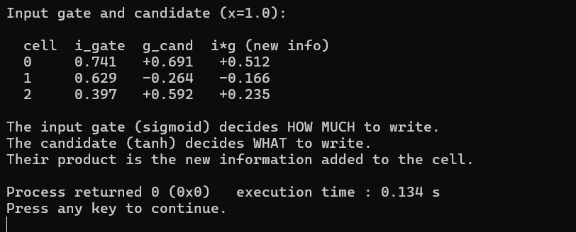
Figure 15-3 computes the gate and the candidate separately and then multiplies them. Cell 1 is the row to look at first, because its candidate comes out at −0.264, a negative number. That is tanh doing the job sigmoid could not, since a candidate restricted to positive values could only ever push the cell state upward and the network would have no way to bring a stored value back down. Being able to write a negative candidate is how the LSTM subtracts without erasing, which is a genuinely different operation from what the forget gate offers.
Cell 2 makes the separation of the two decisions concrete. Its candidate sits at +0.592, which is 86 percent as large as cell 0′s +0.691, so on content alone the two cells are asking to write nearly the same amount. But cell 2′s gate is only 0.397 against cell 0′s 0.741, so what actually lands in the cell is +0.235 against +0.512, less than half as much. The candidate said what, the gate said how much, and the product in the last column is the only number the cell state ever sees.
Notice also that the biases here are all zero, unlike the 1.0 we used on the forget gate. That is deliberate and it follows the same Jozefowicz recommendation. Only the forget gate gets the offset, because only the forget gate needs to start open. An input gate that started open would begin by writing everything it saw straight into memory, which is the opposite of a useful prior, so it starts at sigmoid(0) and lets training decide. The candidate uses tanh because the cell state needs to hold both positive and negative values, which is the same reasoning that put tanh on the hidden state in Chapter 13. The input gate uses sigmoid because it is a switch and its whole job is deciding how much of the candidate to let through, which requires a multiplier bounded between 0 and 1.
One implementation detail worth flagging before we move on. This program collapses the recurrent term to 0.1f * h[k] rather than carrying a full U matrix the way the forget gate listing did, purely to keep the arithmetic visible. A real cell gives i and g their own U_i and U_g matrices exactly as f has U_f, and the complete cell restores them when we assemble it. We now have a value to remove with and a value to write with. Combining them into an actual cell state update takes one line of arithmetic, and that line is the reason the architecture works at all.
15.5 The Cell State Update
We now have a gate that removes and a pair that writes, so combining them into a single update is the last piece of the memory mechanism and it is the heart of the whole architecture.
Read it left to right and the two halves do exactly what the previous two sections built. The old cell state is scaled by the forget gate, which erases whatever is no longer needed and keeps whatever is, and then the new candidate is added on, scaled by the input gate so only the sanctioned fraction of it arrives. Nothing else happens to the cell state at all. There is no weight matrix applied to it, no activation function squashing it, and no transformation of any kind beyond one multiplication and one addition, which is a startlingly small amount of machinery for something that has to carry information across hundreds of time steps.
That plus sign is the whole trick, and it is worth being precise about why. When you differentiate the update with respect to the old cell state, the derivative of f * c_old is simply f and the derivative of the added term is zero, so d(c_new)/d(c_old) comes out as f and nothing more. Compare that against the basic RNN from Chapter 14, where the equivalent quantity was the tanh derivative multiplied by W_h, a product that we measured at 0.19 for a trained unit and which collapsed to 3.76e-15 over twenty steps. Here the per step factor is whatever the forget gate decided, so a gate sitting at 1.0 gives a factor of exactly 1.0, and a signal travelling twenty steps arrives at full strength. Even a fairly leaky gate at 0.9 leaves 0.12 of the gradient after twenty steps, which is thirteen orders of magnitude better than the RNN managed over the same distance.
/* 083_Cell_Update.c */
#include <stdio.h>
#include <math.h>

static float sigmoid(float z)
{
    return 1.0f / (1.0f + expf(-z));
}
static float my_tanh(float z)
{
    if (z < -20) return -1;
    float e = expf(-2 * z);
    return (1 - e) / (1 + e);
}

#define N 3

int main(void)
{
    /* existing cell state */
    float c_old[N] = { 1.0f, -0.5f, 2.0f };

    /* Simulate gate outputs */
    /* forget, keep c[0], erase c[1], keep c[2] */
    float f[N] = { 0.9f, 0.1f, 1.0f };
    /* input, write to c[1], not to c[2] */
    float i_gate[N] = { 0.3f, 0.8f, 0.0f };
    /* candidate values */
    float g[N] = { 0.5f, -0.7f, 0.9f };

    float c_new[N];
    int k;

    for (k = 0; k < N; k++)
        c_new[k] = f[k] * c_old[k] + i_gate[k] * g[k];

    printf("Cell state update: "
           "c_new = f * c_old + i * g\n\n");
    printf("  cell  c_old   f     i     g      "
           "c_new   what happened\n");
    for (k = 0; k < N; k++) {
        printf("  %d     %+5.2f  %.1f   %.1f   "
               "%+.1f   %+5.2f   ",
               k, c_old[k], f[k], i_gate[k],
               g[k], c_new[k]);
        if (f[k] > 0.8f && i_gate[k] < 0.2f)
            printf("kept old value");
        else if (f[k] < 0.2f && i_gate[k] > 0.5f)
            printf("replaced with new");
        else if (f[k] > 0.8f && i_gate[k] > 0.5f)
            printf("kept old + added new");
        else
            printf("partial update");
        printf("\n");
    }

    printf("\nThe '+' is the gradient highway. "
           "During backprop,\n");
    printf("d(c_new)/d(c_old) = f, which is close "
           "to 1 when\n");
    printf("the forget gate is open. The gradient "
           "flows through\n");
    printf("without vanishing.\n");

    return 0;
}
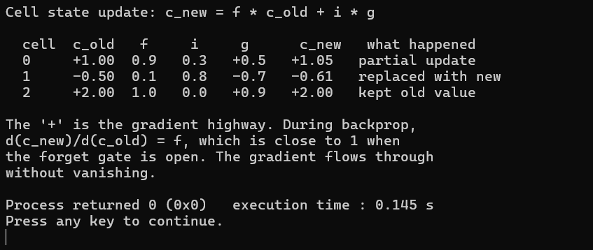
Figure 15-4 takes three cells down three different paths through the same update equation. The three rows are chosen to show the three behaviors the update can produce, and reading them against the equation is the fastest way to see how much range one line of arithmetic covers. Cell 0 is the ordinary case, where a forget gate of 0.9 keeps most of the old +1.00 and leaves +0.900, while an input gate of 0.3 admits only a fraction of the +0.5 candidate and adds +0.150, giving +1.05 in total. Cell 1 is a replacement, because a forget gate of 0.1 wipes out nine tenths of the old −0.50 and leaves only −0.050 behind, while an input gate of 0.8 lets most of the −0.7 candidate through as −0.560, so the −0.61 the cell ends up holding is almost entirely new information. Cell 2 is pure retention, with the forget gate wide open at 1.0 and the input gate shut at 0.0, so the old +2.00 passes through untouched and nothing whatsoever is written.
Cell 2 is the row that matters most for the argument this chapter is making. A value of +2.00 arrived, and a value of +2.00 left, with no attenuation and no distortion, and if the gates hold those settings the same thing happens at the next step and the step after that. The basic RNN had no configuration of any kind that could do this, because tanh saturates and W_h is applied unconditionally, so a value simply could not survive intact no matter what the network wanted. Notice too that all this happens without any branching in the code. Cell 2 is not skipping the write because of an if statement, it is multiplying the candidate by a gate that happens to be zero, and the difference matters because a multiplication is differentiable and a branch is not.
One thing the table quietly demonstrates is that the cell state is not bounded. Cell 2 holds +2.00, which is outside the range tanh could ever produce, and nothing in the update equation will pull it back inside. That is deliberate, since a memory that saturates is a memory that stops distinguishing between large values, and it is also why the hidden state needs its own treatment rather than simply being handed the cell state directly. Squashing has to happen somewhere before the rest of the network sees this, and deciding where and how much is what the output gate does next.
15.6 The Output Gate
The cell state is internal, and nothing outside the cell has any business reading it directly, so the last piece of the architecture is the part that decides how much of that memory to show.
That line does two jobs, and separating them is the fastest way to understand it. The cell state is first passed through tanh, which bounds it to the interval −1 to +1, and then the bounded result is scaled by the output gate o, a sigmoid exactly like the other two. The tanh is there because the cell state is unbounded, as we saw when cell 2 quite happily held +2.00, and anything downstream that expects activations in a sensible range would misbehave if handed values of arbitrary size. The gate is there because there is a real difference between knowing something and saying it, and the LSTM is built so the network can do the first without doing the second.
/* 084_Output_Gate.c */
#include <stdio.h>
#include <math.h>

static float sigmoid(float z)
{
    return 1.0f / (1.0f + expf(-z));
}
static float my_tanh(float z)
{
    if (z < -20) return -1;
    float e = expf(-2 * z);
    return (1 - e) / (1 + e);
}

#define N 3

int main(void)
{
    float c[N] = { 1.5f, -0.3f, 2.8f };
    /* cell state */

    /* Output gate,
       o = sigmoid(W_o * x + U_o * h_prev + b_o) */
    float o[N] = { 0.9f, 0.2f, 0.7f };

    float h[N];
    int k;

    for (k = 0; k < N; k++)
        h[k] = o[k] * my_tanh(c[k]);

    printf("Output gate: h = o * tanh(c)\n\n");
    printf("  cell  c       tanh(c)  o      h\n");
    for (k = 0; k < N; k++)
        printf("  %d     %+5.2f   %+5.3f   %.1f   "
               "%+6.3f\n",
               k, c[k], my_tanh(c[k]), o[k], h[k]);

    printf("\nCell 1 has useful information "
           "(c=-0.3) but the output\n");
    printf("gate is nearly closed (o=0.2), so "
           "h[1] is small.\n");
    printf("The LSTM is choosing not to expose "
           "this information yet.\n");
    printf("It might be needed later.\n");

    return 0;
}
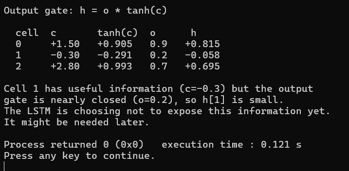
Figure 15-5 holds the cell state fixed and varies the output gate, and the hidden states come out wildly different. Cell 1 is the row the program itself draws attention to, and it is the clearest illustration in the chapter of why the hidden state and the cell state had to be split apart. The cell holds −0.30, which is real information the network worked to put there, but the output gate sits nearly closed at 0.2 so only −0.058 of it reaches the hidden state and the rest of the network sees essentially nothing. The memory has not been damaged in any way, it is simply not being shown, and at the next step the forget gate will find the full −0.30 waiting exactly where it was left. Compare that against the basic RNN of Chapter 13, where h was the memory rather than a view of it, so the only way to hide something from the output layer was to remove it from the state entirely and lose it for good.
Cell 2 shows the other half of the arrangement, and it is where the unbounded cell state from the previous section finally has consequences. The cell holds +2.80, which tanh crushes down to +0.993, and cell 0 holding a much smaller +1.50 comes out at +0.905 for comparison. Internally those two cells are nearly a factor of two apart and the cell state has no trouble at all telling them apart, but after tanh they sit only nine hundredths from each other and the hidden state has lost almost all of that distinction. Push the cell higher and it gets worse, since tanh(4.0) is 0.9993 and tanh(6.0) rounds to 1.0000 at four decimal places, so any two cell values above about four are indistinguishable once the hidden state sees them.
That looks like a flaw and it is actually the reason the design works. The cell state keeps its full range because it is the thing that has to accumulate over hundreds of steps, and a bounded accumulator would saturate and stop counting long before it got there. The hidden state gives up that range because it feeds ordinary weight matrices and activation functions downstream, all of which behave far better with inputs near zero. Trying to serve both requirements with one vector was exactly the compromise that made the basic RNN forget, and the LSTM refuses the compromise by keeping two vectors and converting between them at this one point.
One last thing to notice is what the output gate does to the gradient, because it does not sit on the highway. The path from c_old to c_new runs through the forget gate and the addition, untouched by anything here, while o and the tanh sit on a branch leading out to the hidden state. Gradient arriving from the output layer does get attenuated on its way in through that branch, but the long range flow along the cell state is not affected by how open or closed the output gate happens to be. Storage and exposure are separated in the backward pass just as cleanly as they are in the forward pass, and that separation is what we assemble next, since all four pieces are now built and tested in isolation and the only thing left is to run them together in one structure.
15.7 The Complete LSTM Cell
Everything up to here has been a piece in isolation, so the job now is to put all four into one structure and run a real sequence through it. The cell we are assembling has four gates rather than the one weight matrix a basic RNN carried, and each gate needs its own input weight, its own recurrent matrix, and its own bias, which is why the struct at the top of the listing is four times the size of anything in Chapter 13. The sequence is chosen to be awkward on purpose. A single 1 arrives at step 0, then seven steps of nothing at all, then a second 1 at step 8, which asks the cell to hold on to something across a long stretch where no input is telling it anything.
/* 085_Lstm_Cell.c */
#include <stdio.h>
#include <math.h>
#include <stdlib.h>

static float sigmoid(float z)
{
    return 1.0f / (1.0f + expf(-z));
}
static float my_tanh(float z)
{
    if (z < -20) return -1;
    float e = expf(-2 * z);
    return (1 - e) / (1 + e);
}
static float randf(void)
{
    return (float)rand() / RAND_MAX;
}

#define N 4  /* cell/hidden size */

typedef struct {
    /* Four gates, each with an input weight,
       a recurrent weight and a bias */
    float W_f[N], U_f[N][N], b_f[N];  /* forget */
    float W_i[N], U_i[N][N], b_i[N];  /* input */
    float W_o[N], U_o[N][N], b_o[N];  /* output */
    float W_g[N], U_g[N][N], b_g[N];  /* candidate */
    /* Output projection */
    float W_y[N];
    float b_y;
}
LSTM;

static void lstm_step(const LSTM *l, float x,
                       const float h_prev[N],
                       const float c_prev[N],
                       float h_new[N], float c_new[N])
{
    float f[N], ig[N], o[N], g[N];
    int i, j;

    for (i = 0; i < N; i++) {
        float zf = l->b_f[i] + l->W_f[i] * x;
        float zi = l->b_i[i] + l->W_i[i] * x;
        float zo = l->b_o[i] + l->W_o[i] * x;
        float zg = l->b_g[i] + l->W_g[i] * x;

        for (j = 0; j < N; j++) {
            zf += l->U_f[i][j] * h_prev[j];
            zi += l->U_i[i][j] * h_prev[j];
            zo += l->U_o[i][j] * h_prev[j];
            zg += l->U_g[i][j] * h_prev[j];
        }

        f[i] = sigmoid(zf);
        ig[i] = sigmoid(zi);
        o[i] = sigmoid(zo);
        g[i] = my_tanh(zg);

        /* Cell update: c = f * c_old + i * g */
        c_new[i] = f[i] * c_prev[i] + ig[i] * g[i];

        /* Hidden state: h = o * tanh(c) */
        h_new[i] = o[i] * my_tanh(c_new[i]);
    }
}

static float lstm_output(const LSTM *l,
    const float h[N])
{
    float y = l->b_y;
    int i;
    for (i = 0; i < N; i++)
        y += l->W_y[i] * h[i];
    return y;
}

static void lstm_init(LSTM *l)
{
    int i, j;
    for (i = 0; i < N; i++) {
        /* forget bias = 1 */
        l->W_f[i] = randf()*0.2f-0.1f;
        l->b_f[i] = 1.0f;
        l->W_i[i] = randf()*0.2f-0.1f;
        l->b_i[i] = 0.0f;
        l->W_o[i] = randf()*0.2f-0.1f;
        l->b_o[i] = 0.0f;
        l->W_g[i] = randf()*0.2f-0.1f;
        l->b_g[i] = 0.0f;
        l->W_y[i] = randf()*0.4f-0.2f;
        for (j = 0; j < N; j++) {
            l->U_f[i][j] = randf()*0.2f-0.1f;
            l->U_i[i][j] = randf()*0.2f-0.1f;
            l->U_o[i][j] = randf()*0.2f-0.1f;
            l->U_g[i][j] = randf()*0.2f-0.1f;
        }
    }
    l->b_y = 0;
}

int main(void)
{
    LSTM l;
    float h[N] = {0}, c[N] = {0};
    float h_new[N], c_new[N];
    float seq[] = { 1, 0, 0, 0, 0, 0, 0, 0, 1, 0 };
    int len = 10;
    int t, i;

    srand(42);
    lstm_init(&l);

    printf("LSTM cell processing a sequence:\n");
    printf("(First bit is 1, then zeros, "
           "then another 1)\n\n");
    printf("  t  x  h[0]    c[0]    c[1]    output\n");
    printf("  -- -- ------  ------  ------  ------\n");

    for (t = 0; t < len; t++) {
        lstm_step(&l, seq[t], h, c, h_new, c_new);
        float y = lstm_output(&l, h_new);

        printf("  %2d  %.0f  %+.3f  %+.3f  %+.3f  "
               "%+.3f\n",
               t, seq[t], h_new[0], c_new[0],
                   c_new[1], y);

        for (i = 0; i < N; i++) {
            h[i] = h_new[i];
            c[i] = c_new[i];
        }
    }

    printf("\nWatch the cell state (c[0], c[1]). "
           "Unlike the basic\n");
    printf("RNN hidden state, the cell state "
           "decays far more slowly\n");
    printf("across zero-input steps, because the "
           "forget gate starts\n");
    printf("at sigmoid(1.0), which is 0.73 rather "
           "than 0.\n");

    return 0;
}
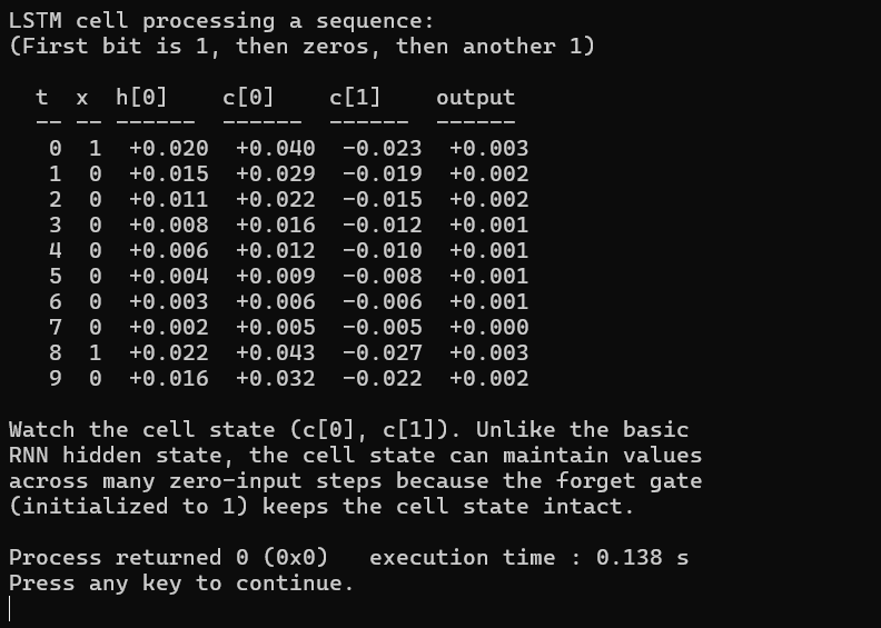
Figure 15-6 carries a value across seven empty steps. Follow c[0] down the column and the shape of the decay is the thing to measure rather than the individual numbers. The first input drives it to +0.040, and across the seven zero steps that follow it drops to +0.029, +0.022, +0.016, +0.012, +0.009, +0.006 and finally +0.005, which works out to about 0.74 of the previous value at every step. That number should look familiar, because it is sigmoid(1.0) and it is the forget gate sitting exactly where the bias put it at initialization. Nothing has trained yet, so the gate has not learned anything about this task, and what you are watching is the untouched initial condition from the forget gate playing out over ten steps of arithmetic.
Be careful about what that does and does not show. The cell state is not being held intact, it is decaying at 26 percent a step, and after seven empty steps only about an eighth of the original value survives. What matters is the comparison rather than the absolute retention, because a basic RNN in the same state would be far worse off. Its hidden state runs through tanh of a small random W_h at every step, so with no input arriving the value collapses toward zero within one or two steps instead of eight, and there is no configuration of the weights that changes that. The LSTM at 0.74 per step is a vastly slower leak, and once the forget gate is trained it can push toward 1.0 and stop leaking almost entirely, which is a possibility the RNN architecture never has.
Now look at what happens when the second 1 arrives at step 8, because that single row is the whole point of the exercise. The cell state jumps to +0.043, which is slightly higher than the +0.040 the first 1 produced back at step 0, and the reason is that the cell was not starting from zero this time. It still held +0.005 left over from the first input, the forget gate kept about 0.74 of that, and the new information landed on top of the residue. Work it through and 0.74 times 0.005 plus 0.040 comes to 0.043, which is what the program printed. Eight steps and seven empty inputs later, the cell remembers that something happened at the beginning, and that memory measurably changes the value it produces.
The two cell columns are also worth comparing against each other, since they decay at visibly different rates. c[0] falls at roughly 0.74 a step while c[1] falls at roughly 0.80, and that difference exists because each cell has its own W_f, its own row of U_f and its own bias, so each computes its own forget gate from the same inputs. Even at initialization with random weights the cells are already choosing different retention rates, and training simply sharpens a distinction that the architecture creates for free.
The output column is the least interesting part of the table and it is honest to say so. Every value sits within a whisker of zero because the network is untrained, the output projection weights are random, and there is no task defining what a correct answer would even look like. What we have built and verified here is the mechanism rather than a working model, and putting that mechanism up against a basic RNN on a sequence long enough to separate them is what the next program does.
15.8 LSTM vs RNN on Long Sequences
Everything so far has been the LSTM on its own, so the last experiment puts it directly against the architecture it replaces on the exact task Chapter 14 used to break the basic RNN. The setup is deliberately minimal. A single 1 arrives at step 0, nothing but zeros follows, and at the end we measure how much output the network still produces, because an output of zero means the network has no memory whatsoever of the only informative thing it was ever shown. Both networks are untrained and randomly initialized, and each length is averaged over twenty different random initializations so no single unlucky draw decides the result.
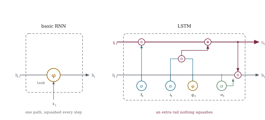
Figure 15-7 puts the two cells side by side with everything but the essential difference stripped out. The RNN on the left has one path from the previous hidden state to the next, and that path runs through tanh, so every step multiplies the gradient by a derivative below 1. Fifty steps means fifty such multiplications, which is the collapse Chapter 14 measured.
The LSTM on the right keeps that path and adds a second one above it. The gates reach up and touch the upper rail, scaling it by f and adding i times g, but nothing squashes it, so a gradient travelling back along that rail is multiplied by the forget gate rather than by a saturating derivative. Hold f near 1 and the rail carries information across many steps almost untouched, which is why the forget gate bias starts at 1.0 in the code.
/* 086_Lstm_Vs_Rnn.c */
#include <stdio.h>
#include <stdlib.h>
#include <math.h>
#include <string.h>

static float sigmoid(float z)
{
    return 1.0f / (1.0f + expf(-z));
}
static float my_tanh(float z)
{
    if (z < -20) return -1;
    float e = expf(-2 * z);
    return (1 - e) / (1 + e);
}
static float randf(void)
{
    return (float)rand() / RAND_MAX;
}

#define N 8
#define MAX_LEN 50

/* --- Basic RNN --- */
typedef struct {
    float W_x[N], W_h[N][N], b_h[N], W_y[N], b_y;
}
BasicRNN;

static float rnn_run(const BasicRNN *r,
                     const float *x, int len)
{
    float h[N] = {0}, hn[N];
    int t, i, j;
    for (t = 0; t < len; t++) {
        for (i = 0; i < N; i++) {
            float z = r->b_h[i] + r->W_x[i] * x[t];
            for (j = 0; j < N; j++)
                z += r->W_h[i][j] * h[j];
            hn[i] = my_tanh(z);
        }
        memcpy(h, hn, sizeof(h));
    }
    float y = r->b_y;
    for (i = 0; i < N; i++) y += r->W_y[i] * h[i];
    return y;
}

/* --- LSTM --- */
typedef struct {
    float W_f[N], U_f[N][N], b_f[N];
    float W_i[N], U_i[N][N], b_i[N];
    float W_o[N], U_o[N][N], b_o[N];
    float W_g[N], U_g[N][N], b_g[N];
    float W_y[N], b_y;
}
LSTMNet;

static float lstm_run(const LSTMNet *l,
                      const float *x, int len)
{
    float h[N] = {0}, c[N] = {0}, hn[N], cn[N];
    int t, i, j;
    for (t = 0; t < len; t++) {
        for (i = 0; i < N; i++) {
            float zf = l->b_f[i] + l->W_f[i] * x[t];
            float zi = l->b_i[i] + l->W_i[i] * x[t];
            float zo = l->b_o[i] + l->W_o[i] * x[t];
            float zg = l->b_g[i] + l->W_g[i] * x[t];
            for (j = 0; j < N; j++) {
                zf += l->U_f[i][j] * h[j];
                zi += l->U_i[i][j] * h[j];
                zo += l->U_o[i][j] * h[j];
                zg += l->U_g[i][j] * h[j];
            }
            float f = sigmoid(zf), ig = sigmoid(zi);
            float o = sigmoid(zo), g = my_tanh(zg);
            cn[i] = f * c[i] + ig * g;
            hn[i] = o * my_tanh(cn[i]);
        }
        memcpy(h, hn, sizeof(h));
        memcpy(c, cn, sizeof(c));
    }
    float y = l->b_y;
    for (i = 0; i < N; i++) y += l->W_y[i] * h[i];
    return y;
}

int main(void)
{
    /* Check how well each architecture preserves
       the first input */
    printf("Information preservation test:\n");
    printf("  Input: 1 at t=0, then zeros. Does the "
           "final hidden\n");
    printf("  state still carry information about "
           "the first input?\n\n");

    int lengths[] = { 5, 10, 20, 30, 50 };
    int n_lengths = 5;
    int li, trial;

    printf("  length   RNN h-norm   LSTM h-norm   "
           "ratio\n");
    printf("  ------   ----------   -----------   "
           "-----\n");

    for (li = 0; li < n_lengths; li++) {
        int len = lengths[li];
        float rnn_norm_sum = 0, lstm_norm_sum = 0;
        int n_trials = 20;

        for (trial = 0; trial < n_trials; trial++) {
            srand(42 + trial);

            /* Initialize RNN */
            BasicRNN r;
            int i, j;
            for (i = 0; i < N; i++) {
                r.W_x[i] = randf()*0.4f-0.2f;
                r.b_h[i] = 0;
                r.W_y[i] = randf()*0.4f-0.2f;
                for (j = 0; j < N; j++)
                    r.W_h[i][j] = randf()*0.4f-0.2f;
            }
            r.b_y = 0;

            /* Initialize LSTM */
            LSTMNet l;
            for (i = 0; i < N; i++) {
                l.W_f[i] = randf()*0.2f-0.1f;
                l.b_f[i] = 1.0f;
                l.W_i[i] = randf()*0.2f-0.1f;
                l.b_i[i] = 0;
                l.W_o[i] = randf()*0.2f-0.1f;
                l.b_o[i] = 0;
                l.W_g[i] = randf()*0.2f-0.1f;
                l.b_g[i] = 0;
                l.W_y[i] = randf()*0.4f-0.2f;
                for (j = 0; j < N; j++) {
                    l.U_f[i][j] = randf()*0.2f-0.1f;
                    l.U_i[i][j] = randf()*0.2f-0.1f;
                    l.U_o[i][j] = randf()*0.2f-0.1f;
                    l.U_g[i][j] = randf()*0.2f-0.1f;
                }
            }
            l.b_y = 0;

            /* Sequence: 1 followed by zeros */
            float x[MAX_LEN] = {0};
            x[0] = 1.0f;

            float ry = rnn_run(&r, x, len);
            float ly = lstm_run(&l, x, len);

            rnn_norm_sum += fabsf(ry);
            lstm_norm_sum += fabsf(ly);
        }

        float rnn_avg = rnn_norm_sum / n_trials;
        float lstm_avg = lstm_norm_sum / n_trials;
        printf("  %3d      %.3e    %.3e   ", len,
               rnn_avg, lstm_avg);
        if (rnn_avg > 0)
            printf("%.0fx\n", lstm_avg / rnn_avg);
        else
            printf("RNN is zero\n");
    }

    printf("\nThe LSTM output norm stays much higher "
           "across long\n");
    printf("sequences. It preserves information "
           "from t=0 because\n");
    printf("the forget gate (bias=1) slows the "
           "decay dramatically.\n");

    return 0;
}
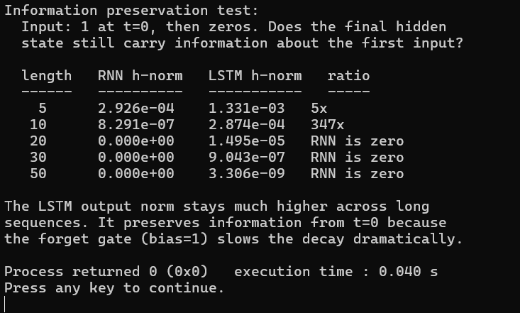
Figure 15-8 measures how much of the first input survives to the end, for both architectures. The first two rows are the ones where the comparison is still meaningful, because they are the only lengths at which the RNN has anything left to measure. At length 5 the two are close enough to look like siblings, with the RNN at 2.926e-04 and the LSTM at 1.331e-03, a gap of only about five times. Five more steps changes the picture completely. By length 10 the RNN has fallen to 8.291e-07, having lost more than 99.7 percent of what it had, while the LSTM sits at 2.874e-04 having lost roughly four fifths, and the gap has widened to 347 times. The two architectures are not decaying at slightly different rates, they are decaying at rates that diverge from each other the further you go.
Put numbers on those rates and the mechanism is unmistakable. The RNN loses about 69 percent of its signal per step, since dropping from 2.926e-04 to 8.291e-07 across five steps works out to a factor of 0.31 each time. The LSTM loses about 26 percent per step, a factor of roughly 0.74, and that number should be familiar by now because it is sigmoid(1.0) again, the forget gate sitting exactly where the initialization bias put it. Check it across the whole table and it barely moves, coming out at 0.736 between lengths 5 and 10, then 0.744, then 0.755 twice more out to length 50. One constant governs the entire decay curve, and it is a constant we chose deliberately back when we built the forget gate.
From length 20 onward the RNN column reads zero, and that needs saying plainly rather than being glossed over. The value has not merely become small, it has underflowed the float representation entirely and there is nothing left to divide by, which is why the ratio column reports that the RNN is zero instead of printing a number. That is the strongest result in the table rather than a missing one. Meanwhile the LSTM at length 20 still carries 1.495e-05, at length 30 it holds 9.043e-07, and even at length 50 there is 3.306e-09 of measurable signal traceable to an input that arrived forty nine steps earlier.
Be clear about what this does and does not prove, because the honest reading is more useful than the triumphant one. The LSTM is also decaying, and 3.306e-09 is not a number you would want to build anything on, so nobody should walk away thinking an untrained LSTM preserves memory indefinitely. The difference is in the exponent rather than the outcome at any single length. Compounding 0.74 across fifty steps leaves you around 2.9e-07 of the original, while compounding 0.31 across the same fifty steps leaves 3.7e-26, and those two numbers are nineteen orders of magnitude apart. One of them is a small signal that a trained output layer can still work with, and the other one is indistinguishable from having never seen the input at all.
The last point is the one that matters most for what comes next. These forget gates are untrained, sitting at their initialized value of 0.74 because nothing has taught them otherwise, and training pushes them wherever the task requires. A gate that learns to sit at 0.99 decays by one percent a step rather than twenty six, which puts 0.6 of the signal at step fifty instead of 2.9e-07. That option exists for the LSTM and does not exist for the basic RNN at all, because there is no weight setting in a basic RNN that stops tanh saturating and stops W_h being applied at every step. The LSTM is not merely better here, it has a knob the other architecture never had.
15.9 The Parameter Cost
Everything the LSTM buys you comes at a price and the price is paid in weights. A basic RNN carries one set of parameters for its single state update, while an LSTM carries four, one each for the forget gate, the input gate, the output gate and the candidate, and every one of those four needs its own input weight matrix, its own recurrent matrix and its own bias vector. Nothing is shared between them, which is the point, because gates that shared weights would be forced to make the same decision.
Counting the recurrent core for a hidden size of N and an input size of M gives the basic RNN three pieces, N*M for the input weights, N*N for the recurrent weights and N for the bias.
The LSTM computes that same quantity four times over, once per gate.
Put real sizes into those and the growth is easier to feel than to read off an algebraic expression.
| Hidden size N | Input size M | Basic RNN | LSTM |
|---|---|---|---|
| 64 | 64 | 8,256 | 33,024 |
| 128 | 64 | 24,704 | 98,816 |
| 256 | 128 | 98,560 | 394,240 |
One thing those formulas quietly leave out is the output layer, and that omission is easy to get wrong because the temptation is to multiply it by four along with everything else. The projection from hidden state to prediction costs N weights plus one bias, and there is only ever one of it regardless of how many gates sit underneath. So for N of 128 and M of 64 the honest totals are 24,833 for the RNN and 98,945 for the LSTM, once you add those 129 parameters to each. If you fold the output layer into the per gate count and then quadruple the lot you will overcount by 387, which is small enough to slip past and wrong all the same. Chapter 12 counted the output layer when it reported 29 parameters for a four unit cell, so that is the convention the rest of the book follows.
The cost is not only memory either. Four gates mean four matrix multiplies where the RNN did one, so the arithmetic per time step is roughly four times heavier as well, and unlike a feedforward layer you pay it once for every element in the sequence. A fifty step sequence through a 128 unit LSTM does two hundred matrix multiplies in the recurrent core against the RNN’s fifty. The elementwise operations, the multiplications by gates and the additions into the cell state, are cheap by comparison and barely register next to the matrix work.
Is four times the model worth it? The comparison above answered that in numbers rather than opinion. At length 20 the RNN output had underflowed to zero while the LSTM still carried 1.495e-05, and no amount of extra training or tuning recovers a signal that has left the float representation. Four times the parameters buys a capability rather than an incremental improvement, which is a different kind of trade from the usual bigger-is-slightly-better bargain. When the dependency you care about spans more than a handful of steps, the basic RNN is not a cheaper option, it is a non-option. That said, four gates is not obviously the minimum. Chapter 16 builds the GRU, which merges the forget and input gates into one and folds the cell state back into the hidden state, arriving at three parameter sets instead of four for roughly seventy five percent of the cost. Whether it matches the LSTM depends on the task, and the comparison there is a good deal closer than the one we just ran.
At N = 128 and M = 64 the RNN comes to 24,705 and the LSTM to 98,820. The LSTM uses 4x more memory and compute per step, but it can learn dependencies that the basic RNN simply cannot.
15.10 Key Takeaways
The LSTM carries two state vectors rather than one. The cell state c is long-term memory that moves from step to step almost untouched, and the hidden state h is short-term working memory derived from it and shown to the rest of the network.
Three sigmoid gates control the flow. The forget gate decides what to erase, the input gate decides how much to write, and the output gate decides how much to expose. Each produces a value between 0 and 1 per element, so different cells receive different decisions from the same input.
The candidate g is not a gate. It uses tanh rather than sigmoid because its job is producing content rather than controlling a valve, and its output can be negative so the network can lower a stored value instead of only raising it.
The cell state update c_new = f * c_old + i * g is additive. Differentiating it with respect to c_old gives f and nothing else, with no weight matrix and no tanh derivative in the way, which is the gradient highway that solves the vanishing gradient problem.
That per step factor is whatever the forget gate holds, so it is not automatically 1. A gate at its initialized value of sigmoid(1.0) gives 0.74 and still loses 26 percent per step, which we measured directly on the complete cell. Training is what pushes the gate toward 1 and stops the leak, and the point is that the LSTM has that option at all.
The forget gate bias is initialized to 1.0, following Jozefowicz et al 2015, and KANN does the same. Left at 0 the gate would start at 0.5 and halve the cell state every step, reaching 8.9e-16 over fifty steps, which is the same order as the basic RNN failure from Chapter 14.
Only the forget gate gets that offset. The input and output gates start at sigmoid(0), because a gate that begins open would write everything it encountered straight into memory.
The recurrent core costs 4 * N * (M + N + 1) parameters against the RNN’s N * (M + N + 1), so four times as many. The output projection is shared across the gates and adds N + 1 once rather than four times, which is easy to get wrong.
We measured what that buys. At length 20 the basic RNN output had underflowed to zero while the LSTM still carried 1.495e-05, so the four times cost purchases a capability rather than an incremental gain.
Tanh for content, sigmoid for control, which is the same pairing Chapter 13 established. Tanh belongs on the cell state and the candidate because both need negative values, and sigmoid belongs on every gate because a multiplier that inverts or amplifies is not a switch.
15.11 Exercises
Before running anything, predict what 085_Lstm_Cell.c will do over 100 steps. The forget gate sits at sigmoid(1.0), so the cell state should fall by roughly 0.74 each step and land near 8.4e-14 of its starting value by step 100. Now modify 085_Lstm_Cell.c to run that long with a 1 at t=0 and zeros afterward, and print c[0] every tenth step. How close was the prediction, and at which step does the value stop being distinguishable from zero in a float?
Change the forget gate bias in 085_Lstm_Cell.c from 1.0 to 0.0 and rerun. The gate now starts at sigmoid(0), which is 0.5, so predict the decay before you look. Compare how many steps the cell state survives against the run you just did, and confirm the ratio between consecutive values matches the gate value in both cases.
Count the parameters in an LSTM with hidden size 64 and input size 32, then do the same for a basic RNN of the same shape. Work out the recurrent core first and add the output projection separately, remembering that the projection is shared rather than repeated once per gate. Check your answer against the formulas at the end of the chapter.
In 081_Forget_Gate.c, find an input that makes all three cells report keep at once. W_f is set to −2.0, 1.0 and 0.5, so cell 0 wants a negative input and cell 1 wants a positive one. Can any single input satisfy both? Explain what that tells you about what a single gate vector can and cannot express in one step.
Implement BPTT for the LSTM. The gradient through the cell state is dc/dc_prev = f, which is the whole reason the architecture works, while the gradient through each gate involves the sigmoid derivative. This is heavier than the basic RNN from Chapter 13 but follows the same chain rule, so start by writing out the four gate gradients on paper before touching any code.
Train the LSTM on the bit counting task from Chapter 13 and compare convergence against the basic RNN, paying particular attention to sequences longer than 20 steps. Watch what the forget gate values do during training, since we argued that training pushes them toward 1 and this is where you get to check that claim.
Read the LSTM implementation in KANN’s kann.c. Find the four gate sets for i, f, o and g, the additive cell update, and the two recurrence links where c->pre is wired to c0 and out->pre is wired to h0. Compare the structure against your 085_Lstm_Cell.c and note where KANN does something you did not.