GRU
Simplified LSTM, two gates instead of three
16.1 What You Will Learn
Chapter 15 built an architecture that works and charged four gate sets and two state vectors for it. The obvious question is whether all of that machinery is necessary, and the Gated Recurrent Unit is the best known attempt at an answer. Cho and colleagues introduced it in 2014, seventeen years after the LSTM, and the design is a deliberate simplification rather than a fresh idea. It merges the cell state and the hidden state back into a single vector, collapses the forget and input gates into one, and drops the output gate entirely, arriving at two gates where the LSTM had three and roughly seventy five percent of the parameter count.
Whether that trade is worth taking is the question this chapter answers with measurements rather than assertions. We build the update gate first, then the reset gate, then assemble a complete cell, then run all three architectures side by side on the same information preservation task Chapter 15 used, and finally count what each one costs in parameters and multiplies. The GRU is also what KANN reaches for in its rnn-bit example, so it is the architecture you would actually deploy if you were building on that library.
16.2 The Simplification
Start from what the LSTM keeps and ask which parts are load bearing. It holds two state vectors, the cell state carrying long-term memory and the hidden state carrying a filtered view of it, and it runs three gates plus a candidate over them. The GRU makes two cuts. It merges the two state vectors into a single h, which removes the output gate along with them because there is no longer an internal value that needs filtering before it is shown. Then it observes that the forget and input gates in an LSTM are usually doing complementary work, keeping less of the old when writing more of the new, and replaces the pair with one gate that does both.
What survives is the update gate z, which decides how much of the old state to keep, and the reset gate r, which decides how much of the old state is visible while the candidate is being computed. Those two gates and the candidate itself give the four equations that define the architecture.
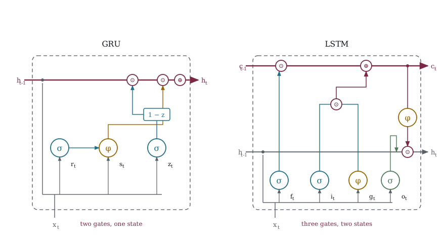
Figure 16-1 puts the two cells side by side. The LSTM on the right runs two rails, a cell state that nothing squashes and a hidden state read off it through the output gate, and it needs three gates to manage that arrangement. The GRU on the left throws away the second rail entirely, so there is one state, no output gate, and nothing left to decide how much of the memory to expose because the memory is the output.
The update gate does the work the forget and input gates did between them. Where the LSTM scales the old cell state by f and separately adds i times the candidate, the GRU uses one number for both sides, keeping z of the old state and 1 minus z of the new. The two proportions are forced to sum to 1, which is a real constraint the LSTM does not have, and it is most of the parameter saving.
The reset gate is the one with no LSTM counterpart. It sits before the candidate rather than after it, deciding how much of the previous state the candidate is even allowed to see while it is being computed.
The last line is the one that carries the architecture and it deserves a moment. It is a straight interpolation between what was already there and what has just been proposed, so a z of 1 leaves the state exactly as it was, a z of 0 discards the old state and installs the candidate wholesale, and anything between blends the two in fixed proportion. Compare that against the LSTM update from the last chapter, where f and i were free to move independently and could both sit high at once, keeping the old value while also adding a large new one. The GRU cannot do that. Its z appears twice in the same line, once as z and once as one minus z, so the two decisions are locked together by construction.
One detail the two gate description hides is that the candidate s carries its own weights, W_s and U_s and b_s, exactly as the gates do. That is why the GRU costs three parameter sets rather than two, and it is what makes the saving against the LSTM twenty five percent rather than fifty. We do that arithmetic properly at the end of the chapter.
Let us build the pieces.
16.3 The Update Gate
The update gate is the whole retain-or-replace decision in one number, so the clearest way to meet it is to hold the old state and the candidate fixed and sweep z across its range to watch what comes out.
/* 087_Update_Gate.c */
#include <stdio.h>
#include <math.h>

static float sigmoid(float z)
{
    return 1.0f / (1.0f + expf(-z));
}

int main(void)
{
    /* Demonstrate the interpolation
       h = z * h_old + (1-z) * s */
    float h_old = 0.8f;    /* existing state */
    float s     = -0.3f;   /* new candidate */

    float z_values[] = { 0.0f, 0.2f, 0.5f, 0.8f, 1.0f };
    int n = 5;
    int i;

    printf("Update gate interpolation: "
           "h = z * h_old + (1-z) * s\n");
    printf("  h_old = %.1f, candidate s = %.1f\n\n",
           h_old, s);
    printf("  z      h_new    interpretation\n");
    printf("  -----  ------   ------------------------"
           "----------------\n");

    for (i = 0; i < n; i++) {
        float z = z_values[i];
        float h_new = z * h_old + (1.0f - z) * s;
        printf("  %.1f    %+.3f   ", z, h_new);

        if (z > 0.9f)
            printf("keep old state (no update)");
        else if (z < 0.1f)
            printf("replace with candidate "
                   "(full update)");
        else if (z > 0.6f)
            printf("mostly keep, small update");
        else if (z < 0.4f)
            printf("mostly replace, small retention");
        else printf("equal blend");
        printf("\n");
    }

    printf("\nCompare to LSTM. The forget gate and "
           "input gate are\n");
    printf("independent. f can be 0.9 and i can be "
           "0.9 at once,\n");
    printf("meaning the LSTM can both keep the old "
           "AND add the new.\n");
    printf("The GRU couples them, so keeping more "
           "old means adding less new.\n");

    return 0;
}
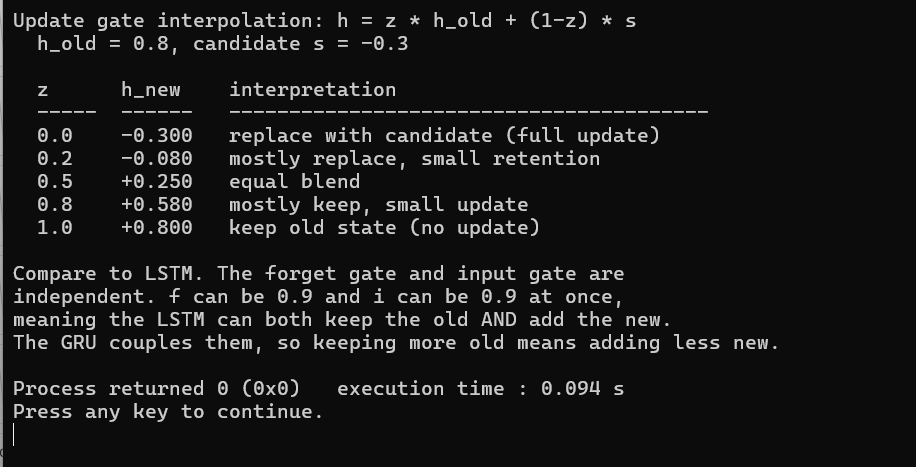
Figure 16-2 interpolates between the old state and the candidate. The old state is +0.8 and the candidate is −0.3, which are deliberately far apart and on opposite sides of zero so the blending is easy to follow. At z of 0.0 the output is exactly the candidate, −0.300, and the old state has been discarded without trace. At z of 1.0 the output is exactly the old state, +0.800, and the candidate has been ignored completely. Between those two ends the values move smoothly and linearly, so z of 0.5 gives +0.250, which is the midpoint of +0.8 and −0.3, and z of 0.8 gives +0.580, which is four fifths of the way back toward the old value. Nothing here is squashed or saturated, because interpolation is a straight line rather than a curve.
The closing text is where the trade-off gets stated and it is worth taking seriously rather than reading past. An LSTM could set f to 0.9 and i to 0.9 in the same step, keeping nearly all of its old cell value while also adding nearly all of a new candidate on top, and the cell state would grow because nothing forces the two to sum to anything in particular. The GRU cannot express that at all. Its two coefficients are z and one minus z, which always sum to exactly 1, so keeping eighty percent of the old state means the candidate can contribute at most twenty percent. Retention and acquisition compete for a fixed budget.
Whether that costs you anything depends on the task. It rules out an LSTM behavior that is occasionally useful, where a cell accumulates rather than blends, but it also makes the state naturally bounded, since a convex combination of two values in a range stays in that range. The LSTM needed an unbounded cell state and a tanh on the way out to manage the same problem, which is machinery the GRU simply does not require.
16.4 The Reset Gate
The update gate decides how much history to keep, and the reset gate decides something quite different, which is how much history the candidate is allowed to look at while it is being computed. Those sound similar and are not. One controls what survives, the other controls what informs the replacement.
/* 088_Reset_Gate.c */
#include <stdio.h>
#include <math.h>

static float my_tanh(float z)
{
    if (z < -20) return -1;
    float e = expf(-2 * z);
    return (1 - e) / (1 + e);
}

#define N 3

int main(void)
{
    float x = 1.0f;
    float h_prev[N] = { 0.8f, -0.5f, 0.3f };
    float W_s[N] = { 0.5f, -0.3f, 0.7f };
    float U_s[N] = { 0.4f, 0.6f, -0.2f };
    float b_s[N] = { 0, 0, 0 };
    int i;

    printf("Reset gate effect on the candidate:\n");
    printf("  s = tanh(W_s * x + U_s * "
           "(r * h_prev) + b_s)\n\n");
    printf("  h_prev = [%.1f, %.1f, %.1f]\n\n",
           h_prev[0], h_prev[1], h_prev[2]);

    float r_values[] = { 0.0f, 0.5f, 1.0f };
    int n_r = 3;

    for (int ri = 0; ri < n_r; ri++) {
        float r = r_values[ri];
        float s[N];

        for (i = 0; i < N; i++) {
            /* reset gate applied to history */
            float rh = r * h_prev[i];
            s[i] = my_tanh(W_s[i] * x
                           + U_s[i] * rh + b_s[i]);
        }

        printf("  r=%.1f: candidate = "
               "[%+.3f, %+.3f, %+.3f]",
               r, s[0], s[1], s[2]);
        if (r < 0.1f) printf("  (ignores history)");
        else if (r > 0.9f)
            printf("  (uses full history)");
        printf("\n");
    }

    printf("\nWhen r=0, the candidate depends only "
           "on the current input.\n");
    printf("This lets the GRU 'reset' and compute "
           "fresh state from\n");
    printf("scratch, useful when the context "
           "changes abruptly.\n");

    return 0;
}
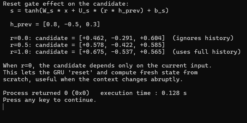
Figure 16-3 computes the candidate with the history fully hidden, half visible and fully visible. Read the three rows against a fixed history of [0.8, −0.5, 0.3] and the gate’s effect is visible in every element. At r of 0.0 the candidate comes out as [+0.462, −0.291, +0.604], and those numbers depend only on the current input and the bias, because r multiplies h_prev before U_s ever sees it and multiplying by zero removes the history entirely. At r of 1.0 the full history is in play and the candidate becomes [+0.675, −0.537, +0.565]. The middle row at r of 0.5 sits between the two, as you would expect.
Notice which direction each element moved. The first element rose from +0.462 to +0.675 as the history was admitted, the second fell from −0.291 to −0.537, and the third actually dropped slightly from +0.604 to +0.565. The history does not push the candidate uniformly in any direction, it pushes each element according to that element’s row of U_s, so a gate value that helps one element can hinder another. This is the same per element independence the LSTM gates showed in Chapter 15, arriving here through a different route.
The reason to want a reset gate at all is abrupt context change. When a sequence turns a corner, at a sentence boundary or a scene change or a new speaker, the accumulated history stops being useful and can actively mislead the candidate. Closing r lets the GRU compute fresh content from the current input alone while the update gate separately decides how much of the old state to keep, and the fact that those are two independent decisions is what makes the reset gate worth its parameters. The LSTM reaches a similar end through its forget gate, but the mechanism differs in a way worth being precise about. The LSTM erases the stored value, while the GRU leaves the stored value alone and merely hides it from the candidate computation.
16.5 The Complete GRU Cell
Both gates and the candidate now go into one structure, and the sequence is the same awkward one Chapter 15 used, a single 1 at step 0 followed by seven empty steps and then a second 1 at step 8.
/* 089_Gru_Cell.c */
#include <stdio.h>
#include <math.h>
#include <stdlib.h>

static float sigmoid(float z)
{
    return 1.0f / (1.0f + expf(-z));
}
static float my_tanh(float z)
{
    if (z < -20) return -1;
    float e = expf(-2 * z);
    return (1 - e) / (1 + e);
}
static float randf(void)
{
    return (float)rand() / RAND_MAX;
}

#define N 4

typedef struct {
    float W_z[N], U_z[N][N], b_z[N];  /* update gate */
    float W_r[N], U_r[N][N], b_r[N];  /* reset gate */
    float W_s[N], U_s[N][N], b_s[N];  /* candidate */
    float W_y[N], b_y;                 /* output */
}
GRU;

static void gru_step(const GRU *g, float x,
                      const float h_prev[N],
                          float h_new[N])
{
    float z[N], r[N], s[N];
    int i, j;

    for (i = 0; i < N; i++) {
        /* Update gate */
        float zz = g->b_z[i] + g->W_z[i] * x;
        /* Reset gate */
        float zr = g->b_r[i] + g->W_r[i] * x;

        for (j = 0; j < N; j++) {
            zz += g->U_z[i][j] * h_prev[j];
            zr += g->U_r[i][j] * h_prev[j];
        }

        z[i] = sigmoid(zz);
        r[i] = sigmoid(zr);

        /* Candidate: uses r * h_prev */
        float zs = g->b_s[i] + g->W_s[i] * x;
        for (j = 0; j < N; j++)
            zs += g->U_s[i][j] * (r[i] * h_prev[j]);
        s[i] = my_tanh(zs);

        /* New state: interpolation */
        h_new[i] = z[i] * h_prev[i]
            + (1.0f - z[i]) * s[i];
    }
}

static void gru_init(GRU *g)
{
    int i, j;
    for (i = 0; i < N; i++) {
        g->W_z[i] = randf()*0.2f-0.1f;
        g->b_z[i] = 0;
        g->W_r[i] = randf()*0.2f-0.1f;
        g->b_r[i] = 0;
        g->W_s[i] = randf()*0.2f-0.1f;
        g->b_s[i] = 0;
        g->W_y[i] = randf()*0.4f-0.2f;
        for (j = 0; j < N; j++) {
            g->U_z[i][j] = randf()*0.2f-0.1f;
            g->U_r[i][j] = randf()*0.2f-0.1f;
            g->U_s[i][j] = randf()*0.2f-0.1f;
        }
    }
    g->b_y = 0;
}

int main(void)
{
    GRU g;
    float h[N] = {0}, h_new[N];
    float seq[] = { 1, 0, 0, 0, 0, 0, 0, 0, 1, 0 };
    int len = 10;
    int t, i;

    srand(42);
    gru_init(&g);

    printf("GRU cell processing a sequence:\n\n");
    printf("  t  x  h[0]    h[1]    h[2]    h[3]\n");
    printf("  -- -- ------  ------  ------  ------\n");

    for (t = 0; t < len; t++) {
        gru_step(&g, seq[t], h, h_new);
        printf("  %2d  %.0f  %+.3f  %+.3f  %+.3f  "
               "%+.3f\n",
               t, seq[t], h_new[0], h_new[1],
               h_new[2], h_new[3]);
        for (i = 0; i < N; i++) h[i] = h_new[i];
    }

    printf("\nThe GRU has one state vector, with no "
           "separate cell state.\n");
    printf("The update gate z controls retention "
           "vs replacement.\n");

    return 0;
}
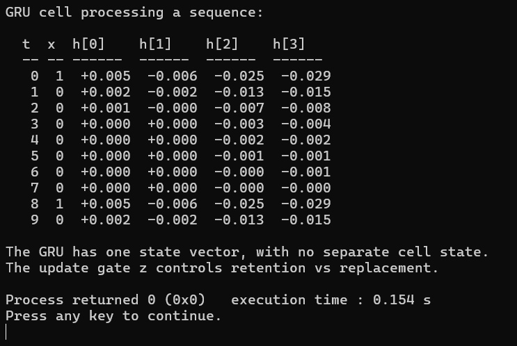
Figure 16-4 runs a complete cell over the same sequence the LSTM saw. Follow h[3] down the column, since it is the element with the largest starting value and therefore the clearest trace. The first input drives it to −0.029, and it then falls to −0.015, −0.008, −0.004, −0.002 and −0.001 before reaching −0.000, which is almost exactly half the previous value at every step. Check the other columns and they do the same thing at their own scale, with h[0] starting smaller at +0.005 and hitting zero by step 3 simply because it had less to lose.
That factor of one half is not an accident. All three biases here are initialized to zero, so z starts at sigmoid(0), and an update gate sitting at exactly 0.5 keeps half the old state and fills the rest with a candidate that is itself near zero at initialization. Compare that against the LSTM from the last chapter, which decayed at 0.74 per step because Chapter 15 deliberately set its forget gate bias to 1.0. The difference between the two is not architectural at all, it is an initialization choice that Chapter 15 made and this GRU does not, and nothing stops you setting b_z to 1.0 here to get the same 0.74. Many GRU implementations do exactly that for exactly that reason.
The consequence shows up at step 8. When the second 1 arrives, h[3] returns to −0.029 and h[0] returns to +0.005, which are precisely the values they took at step 0, and that exact equality is the whole story. The state had already decayed to zero, so the new input landed on nothing and the cell retains no trace whatsoever of the first input. The LSTM in the same experiment reached +0.043 against its earlier +0.040, and that extra 0.003 was the residue of the first input still measurably present eight steps later. This GRU has no residue to add.
Do not read that as the GRU being the weaker architecture, because what you are looking at is a fair comparison of two initializations rather than two designs. It does illustrate something real though, which is that the gradient highway is only ever as open as the gate initialization leaves it, and the comparison ahead measures what happens once both architectures are given the initialization their own chapter recommends.
16.6 GRU vs LSTM vs RNN Side by Side
All three architectures now run on the same information preservation task the last chapter used, with a 1 at step 0, zeros thereafter, and the norm of the final hidden state measured across thirty random initializations at each length. This time every network gets the initialization its own chapter recommended, so the LSTM’s forget gate bias is 1.0 and the GRU’s gates start at zero.
/* 090_Compare.c */
#include <stdio.h>
#include <stdlib.h>
#include <math.h>
#include <string.h>

static float sigmoid(float z)
{
    return 1.0f / (1.0f + expf(-z));
}
static float my_tanh(float z)
{
    if (z < -20) return -1;
    float e = expf(-2 * z);
    return (1 - e) / (1 + e);
}
static float randf(void)
{
    return (float)rand() / RAND_MAX;
}

#define N 8

/* --- Basic RNN --- */
static void rnn_run(const float *x, int len,
    float *h_final)
{
    float W_x[N], W_h[N][N], b[N], h[N] = {0}, hn[N];
    int t, i, j;
    for (i = 0; i < N; i++) {
        W_x[i] = randf()*0.4f-0.2f;
        b[i] = 0;
        for (j = 0; j < N; j++)
            W_h[i][j] = randf()*0.4f-0.2f;
    }
    for (t = 0; t < len; t++) {
        for (i = 0; i < N; i++) {
            float z = b[i] + W_x[i] * x[t];
            for (j = 0; j < N; j++)
                z += W_h[i][j] * h[j];
            hn[i] = my_tanh(z);
        }
        memcpy(h, hn, sizeof(h));
        }
    memcpy(h_final, h, sizeof(h));
}

/* --- LSTM --- */
static void lstm_run(const float *x, int len,
                     float *h_final)
{
    float W[4][N], U[4][N][N], b[4][N];
    float h[N] = {0}, c[N] = {0}, hn[N], cn[N];
    int t, i, j, g;
    for (g = 0; g < 4; g++) for (i = 0; i < N; i++) {
        W[g][i] = randf()*0.2f-0.1f;
        /* gate 0 is forget, and it is the only
           one that starts open */
        b[g][i] = (g == 0) ? 1.0f : 0.0f;
        for (j = 0; j < N; j++)
            U[g][i][j] = randf()*0.2f-0.1f;
    }
    for (t = 0; t < len; t++) {
        for (i = 0; i < N; i++) {
            float zz[4];
            for (g = 0; g < 4; g++) {
                zz[g] = b[g][i] + W[g][i] * x[t];
                for (j = 0; j < N; j++)
                    zz[g] += U[g][i][j] * h[j];
            }
            float fi = sigmoid(zz[0]);
            float ii = sigmoid(zz[1]);
            float oi = sigmoid(zz[2]);
            float gi = my_tanh(zz[3]);
            cn[i] = fi * c[i] + ii * gi;
            hn[i] = oi * my_tanh(cn[i]);
        }
        memcpy(h, hn, sizeof(h));
        memcpy(c, cn, sizeof(c));
    }
    memcpy(h_final, h, sizeof(h));
}

/* --- GRU --- */
static void gru_run(const float *x, int len,
    float *h_final)
{
    float W_z[N], U_z[N][N], b_z[N];
    float W_r[N], U_r[N][N], b_r[N];
    float W_s[N], U_s[N][N], b_s[N], h[N] = {0}, hn[N];
    int t, i, j;
    for (i = 0; i < N; i++) {
        W_z[i] = randf()*0.2f-0.1f;
        b_z[i] = 0;
        W_r[i] = randf()*0.2f-0.1f;
        b_r[i] = 0;
        W_s[i] = randf()*0.2f-0.1f;
        b_s[i] = 0;
        for (j = 0; j < N; j++) {
            U_z[i][j] = randf()*0.2f-0.1f;
            U_r[i][j] = randf()*0.2f-0.1f;
            U_s[i][j] = randf()*0.2f-0.1f;
        }
    }
    for (t = 0; t < len; t++) {
        for (i = 0; i < N; i++) {
            float zz = b_z[i]+W_z[i]*x[t];
            float zr = b_r[i]+W_r[i]*x[t];
            for (j = 0; j < N; j++) {
                zz += U_z[i][j]*h[j];
                zr += U_r[i][j]*h[j];
            }
            float z = sigmoid(zz), r = sigmoid(zr);
            float zs = b_s[i] + W_s[i]*x[t];
            for (j = 0; j < N; j++)
                zs += U_s[i][j]*(r*h[j]);
            float s = my_tanh(zs);
            hn[i] = z * h[i] + (1-z) * s;
            }
        memcpy(h, hn, sizeof(h));
        }
    memcpy(h_final, h, sizeof(h));
}

int main(void)
{
    int lengths[] = { 5, 10, 20, 50 };
    int n_lengths = 4;
    int li, trial, i;

    printf("Information preservation, input 1 at "
           "t=0 then zeros.\n");
    printf("Measure norm of final hidden state.\n\n");
    printf("  length   RNN         GRU         "
           "LSTM\n");
    printf("  ------   ---------   ---------   "
           "---------\n");

    for (li = 0; li < n_lengths; li++) {
        int len = lengths[li];
        float rnn_sum = 0, gru_sum = 0, lstm_sum = 0;
        int n_trials = 30;

        for (trial = 0; trial < n_trials; trial++) {
            srand(42 + trial);

            float x[100] = {0};
            x[0] = 1.0f;
            float h[N];
            float norm;

            srand(42 + trial);
            rnn_run(x, len, h);
            norm = 0;
            for (i = 0; i < N; i++)
                norm += h[i]*h[i];
            rnn_sum += sqrtf(norm);

            srand(42 + trial);
            gru_run(x, len, h);
            norm = 0;
            for (i = 0; i < N; i++)
                norm += h[i]*h[i];
            gru_sum += sqrtf(norm);

            srand(42 + trial);
            lstm_run(x, len, h);
            norm = 0;
            for (i = 0; i < N; i++)
                norm += h[i]*h[i];
            lstm_sum += sqrtf(norm);
        }

        printf("  %3d      %.3e   %.3e   %.3e\n",
               len, rnn_sum/n_trials,
               gru_sum/n_trials, lstm_sum/n_trials);
    }

    printf("\nRNN decays fastest, having no gates.\n");
    printf("GRU retains more, since the update "
           "gate allows pass-through.\n");
    printf("LSTM retains most, with a dedicated "
           "cell state and forget bias 1.\n");

    return 0;
}
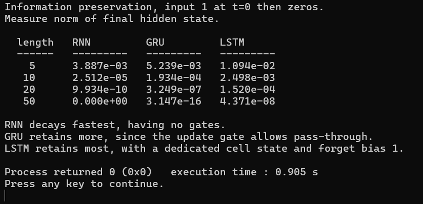
Figure 16-5 measures all three architectures on the same information preservation task. The ordering holds at every length and it is the ordering the architectures predict. At length 5 the RNN sits at 3.887e-03, the GRU at 5.239e-03 and the LSTM at 1.094e-02, so the two gated designs are already ahead but the margin is modest, with the GRU only about a third better than the RNN. Stretch to length 10 and the separation begins in earnest, since the RNN falls to 2.512e-05 while the GRU holds 1.934e-04 and the LSTM holds 2.498e-03, which puts the GRU nearly eight times ahead of the RNN and the LSTM thirteen times ahead of the GRU. By length 20 the RNN is down to 9.934e-10 and effectively finished, while the GRU carries 3.249e-07 and the LSTM carries 1.520e-04.
Length 50 is where the three separate completely. The RNN has underflowed to zero and there is nothing left to measure at all. The GRU holds 3.147e-16, which is a real number rather than zero but far too small for any output layer to do anything useful with. The LSTM holds 4.371e-08, roughly a hundred and forty million times more signal than the GRU across the same distance. That gap is the price of the GRU’s simplification made visible, and it traces directly back to the coupling in the update gate, because a GRU cannot hold z near 1 without simultaneously refusing to write anything new, while an LSTM can pin its forget gate near 1 and still accept input through an entirely separate channel.
Set that against what the simplification buys, which the next section counts, and the honest summary is that the GRU sits much closer to the LSTM than to the RNN. Both gated architectures beat the ungated one by margins that widen with every step of length, and by length 50 the RNN is not in the comparison at all. Choosing between GRU and LSTM is a real decision that depends on how far back your dependencies reach. Choosing either one over a basic RNN for a long sequence is not a decision, it is arithmetic.
16.7 Parameter Count Comparison
The GRU has fewer gates and it is fair to ask exactly how much that saves, which is a question best answered by a program that does the arithmetic rather than by an estimate.
/* 091_Params.c */
#include <stdio.h>

int main(void)
{
    int n = 64;   /* hidden size */
    int m = 32;   /* input size */

    /* W_x + W_h + b */
    int rnn_params = n*m + n*n + n;
    /* z, r and the candidate s */
    int gru_params = 3 * (n*m + n*n + n);
    /* f, i, o and the candidate g */
    int lstm_params = 4 * (n*m + n*n + n);

    printf("Parameter count comparison "
           "(hidden=%d, input=%d):\n\n", n, m);
    printf("  Architecture   Gate sets   Parameters"
           "   Ratio\n");
    printf("  ------------   ---------   ----------"
           "   -----\n");
    printf("  Basic RNN      1           %6d       "
           "1.0x\n", rnn_params);
    printf("  GRU            3           %6d       "
           "%.1fx\n", gru_params,
           (float)gru_params/rnn_params);
    printf("  LSTM           4           %6d       "
           "%.1fx\n", lstm_params,
           (float)lstm_params/rnn_params);

    printf("\n  GRU uses 75%% of LSTM's parameters.\n");
    printf("  On many tasks, GRU matches LSTM "
           "performance.\n");
    printf("  KANN uses GRU for its rnn-bit "
           "example.\n");

    /* multiplies per step, approximately */
    int rnn_per_step = n*m + n*n;
    int gru_per_step = 3 * (n*m + n*n);
    int lstm_per_step = 4 * (n*m + n*n);

    printf("\n  Compute per step (multiplies, "
           "approx):\n");
    printf("    RNN:  %6d\n", rnn_per_step);
    printf("    GRU:  %6d (%.1fx RNN)\n",
           gru_per_step,
           (float)gru_per_step/rnn_per_step);
    printf("    LSTM: %6d (%.1fx RNN)\n",
           lstm_per_step,
           (float)lstm_per_step/rnn_per_step);

    return 0;
}
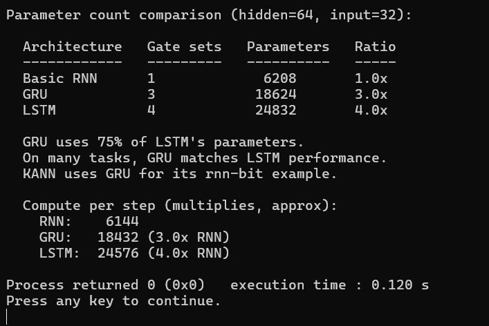
Figure 16-6 counts parameters and multiplies per step for the three. The middle column is the one that catches people out. The GRU is described everywhere as having two gates, and it does, but the table lists three parameter sets because the candidate s carries its own W_s, U_s and b_s just as the gates carry theirs. Counting only z and r would give 12,416 for a hidden size of 64 and an input size of 32, and the real answer is 18,624. The same trap exists on the LSTM side, where three gates plus one candidate makes four sets rather than three.
With that settled the ratios come out clean. A basic RNN needs 6,208 parameters at these sizes, the GRU needs three times that at 18,624 and the LSTM four times that at 24,832, so the GRU costs seventy five percent of an LSTM and three times a plain RNN. The compute figures underneath track the same ratios, since the dominant cost per step is one matrix multiply per parameter set, giving 6,144 multiplies for the RNN, 18,432 for the GRU and 24,576 for the LSTM. Note that these counts cover the recurrent core only, and the output projection adds N plus 1 once to each of them rather than being repeated per gate, which is the same distinction the LSTM count had to make.
Whether saving a quarter is worth anything depends entirely on where the model runs. Twenty five percent off 24,832 parameters is 6,208 floats, which is 24 kilobytes at single precision and irrelevant on a workstation. Scale to a hidden size of 512 and the same twenty five percent is a saving of megabytes, and on a device with a fixed memory budget that is the difference between fitting and not fitting.
16.8 When to Use What
The basic RNN is almost never the right answer. We measured its output at zero by length 50 while both gated architectures still had something, and it offers no way to fix that through training because there is no gate to learn. Reach for it only when sequences are genuinely short, under roughly ten steps, and even then the saving is small enough that the safer choice costs little.
The GRU is a reasonable default when you need recurrence. It is simpler to implement, it runs at three quarters the cost, and on a large fraction of published benchmarks the accuracy difference against an LSTM is within noise. KANN uses it for the sequence examples, which is a practical endorsement from a library that had a free choice.
The LSTM earns its extra quarter when dependencies run long. The length 50 row showed it holding a hundred and thirty million times more signal than the GRU, and that gap comes from the independent forget and input gates rather than from anything incidental, so it will not close with tuning. Speech recognition and machine translation used LSTMs for years on exactly this reasoning, though transformers have since taken most of that ground.
Transformers from Chapter 24 onward beat both on most language tasks today, and they do it by removing the recurrence entirely so that no signal has to survive a per step multiplication at all. What they charge for that is memory and compute that scale with the square of the sequence length, which is a very different cost profile from anything in this chapter. When the compute budget is tight the gated recurrent architectures remain the practical option, and between the two the choice comes down to how far back the dependencies reach.
16.9 Key Takeaways
The GRU has two gates, the update gate z and the reset gate r, against the LSTM’s three. It carries one state vector rather than two, and it has no output gate because there is no internal cell state that needs filtering before it is shown.
The candidate s is not a gate but it does carry its own W_s, U_s and b_s. That is why the GRU costs three parameter sets rather than two, and why the saving against an LSTM is twenty five percent rather than fifty.
The state update h = z * h_prev + (1 - z) * s is an interpolation. The two coefficients always sum to 1, so keeping more of the old state forces the candidate to contribute less, which is the coupling an LSTM avoids by keeping f and i independent.
The reset gate controls what the candidate can see rather than what survives. Closing it computes fresh content from the current input alone while leaving the stored state untouched, which is a different operation from the LSTM erasing its cell.
The gradient path is d(h_new)/d(h_prev) = z plus a term through the candidate, so the highway is as open as z happens to be. At the default initialization z sits at sigmoid(0), which is 0.5, and we measured h[3] falling from −0.029 to −0.000 at almost exactly half per step because of it.
Setting b_z to 1.0 gives the GRU the same starting point Chapter 15 gave the LSTM. Nothing about the architecture prevents it, and the 0.5 decay in 089_Gru_Cell.c is an initialization choice rather than a limitation of the design.
At a hidden size of 64 and an input size of 32 the recurrent cores cost 6,208 for an RNN, 18,624 for a GRU and 24,832 for an LSTM. Compute per step tracks the same ratios, and the output projection adds N plus 1 once to each rather than per gate.
We measured all three at length 50. The RNN underflowed to zero, the GRU held 3.147e-16 and the LSTM held 4.371e-08, which is roughly a hundred and forty million times more. Both gated designs beat the RNN by margins that widen with length, and the LSTM pulls away from the GRU once the sequence runs long enough.
KANN implements the GRU as kann_layer_gru2 and uses z equal to 1 to mean keep the old state. Some texts use the opposite convention, so check which one any implementation follows before comparing gate values against a paper.
16.10 Exercises
Trace the GRU equations by hand for a two step sequence with a hidden size of 2, writing out z, r, s and h at every step. Do it before running anything, then check against 089_Gru_Cell.c with the same weights, because the arithmetic is small enough to verify completely and that is rarer than it sounds.
Set b_z to 1.0 in 089_Gru_Cell.c and rerun. We measured the state halving each step at the default initialization, so predict the new decay rate from sigmoid(1.0) first. Does the second input at step 8 now land on a nonzero residue the way the LSTM did last chapter?
Modify 089_Gru_Cell.c to run 50 steps with a single input at t=0 and compare the decay directly against the LSTM from Chapter 15. Run it once at the default bias and once with b_z at 1.0, and work out how much of the gap between the two architectures is initialization rather than design.
Implement BPTT for the GRU. The gradient through the interpolation is dh/dh_prev = z + (1-z) * ds/dh_prev, and the second term is the awkward one because the candidate sees h_prev through the reset gate. Write out ds/dh_prev on paper before coding, remembering that r is itself a function of h_prev.
Train a GRU on the bit counting task from Chapter 13 and compare convergence against the basic RNN and the LSTM. Print the mean update gate value each epoch, since we argued the gap between GRU and LSTM comes from the coupling in z and this is where you can watch what z actually learns.
Some implementations apply the reset gate as r * (U_s * h_prev) rather than U_s * (r * h_prev). Work out whether the two are equivalent, and if they are not, construct a small example with a 2 by 2 U_s that produces different candidates.
Read KANN’s GRU implementation in kann.c, specifically kann_layer_gru2. KANN uses z equal to 1 to mean keep the old state, and some texts use the opposite convention, so verify which one 089_Gru_Cell.c follows before you compare gate values against any paper.