Bidirectional RNNs
Seeing future and past context
17.1 What You Will Learn
Every recurrent architecture in the last four chapters reads left to right, so at any position the network knows what came before and nothing about what comes after. For a great many tasks that is exactly the wrong constraint. Read the sentence “I went to the bank to deposit money” and the word bank is genuinely ambiguous at the moment you reach it, since a river bank and a financial one are equally plausible until the words deposit money arrive three positions later. A forward-only model has to commit before the disambiguating evidence exists.
The bidirectional wrapper solves this by refusing to choose. It runs two entirely separate recurrent networks over the same sequence, one starting at the left and one starting at the right, then joins their hidden states at each position so that every output sees the whole sequence rather than half of it. Nothing about the cell changes, which is the appeal of the idea, so the same wrapper works over a basic RNN, an LSTM or a GRU without modification.
In this chapter we build both passes, combine them, attach an output layer that labels every position, work out precisely when the approach is unusable, and finish by wrapping GRU cells to build the BiGRU that dominated sequence labelling for years before transformers arrived. The constraint that makes bidirectionality impossible for some tasks turns out to be the same distinction that separates BERT from GPT, so that discussion repays careful reading even though its listing is the simplest in the chapter.
17.2 The Limitation of One Direction
Part-of-speech tagging makes the problem concrete because the ambiguity is lexical rather than subtle. Take the word lead, which is a verb in “they lead the race” and a noun in “the lead pipe” and an adjective in “the lead singer”, with identical spelling in all three. Nothing about the word itself settles the question. In “the lead singer” it is the word to the right that resolves it, since a noun following lead pushes lead into the adjective slot, while in “they lead the race” it is the pronoun to the left doing the work.
A forward-only RNN standing at lead in the first phrase has consumed the and nothing else. Every piece of evidence it needs sits one position to its right, on the other side of a boundary the architecture cannot cross. Training longer does not help, a larger hidden state does not help, and gating does not help, because the information has not arrived yet in any form. This is a different failure from the vanishing gradient of Chapter 14, where the information was present but the gradient could not reach back to it. Here the information is genuinely absent at the moment the decision has to be made.
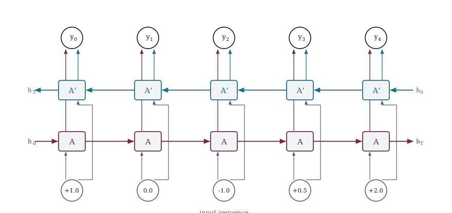
Figure 17-1 shows the fix unrolled, using the five input values the first program in this chapter feeds in. There are two chains rather than one. The forward chain runs left to right exactly as before, and the backward chain runs right to left over the same inputs, starting from its own initial state at the far end of the sequence.
The two chains never touch. No arrow runs between them at any position, and neither one can see the other one’s state, which means the backward pass is not a correction applied to the forward pass but a second independent reading of the same data. They meet only at the output, where each position has both a summary of everything to its left and a summary of everything to its right.
That independence is why the whole thing can be computed with the RNN code already written. Run the existing loop forward over the sequence, run it again backward over the reversed sequence, and pair the results up by position.
17.3 Forward and Backward Passes
The fix is less clever than it sounds. Run one RNN from position 0 up to the end, run a second RNN from the end down to position 0, and keep both sets of hidden states. The two networks carry their own weights and never share a parameter, so the backward network is not the forward network run in reverse, it is a separate model that happens to see the sequence in the opposite order.
/* 092_Two_Directions.c */
#include <stdio.h>
#include <math.h>

static float my_tanh(float z)
{
    if (z < -20) return -1;
    float e = expf(-2 * z);
    return (1 - e) / (1 + e);
}

#define N_HID 2
#define SEQ_LEN 5

/* Simple RNN step,
   h_new = tanh(w_x * x + w_h * h_old + b) */
static void rnn_step(const float w_x[N_HID],
                     const float w_h[N_HID][N_HID],
                     const float b[N_HID], float x,
                     const float h_old[N_HID],
                     float h_new[N_HID])
{
    int i, j;
    for (i = 0; i < N_HID; i++) {
        float z = b[i] + w_x[i] * x;
        for (j = 0; j < N_HID; j++)
            z += w_h[i][j] * h_old[j];
        h_new[i] = my_tanh(z);
    }
}

int main(void)
{
    /* A short sequence of values */
    float seq[SEQ_LEN] = { 1.0f, 0.0f, -1.0f,
        0.5f, 2.0f };

    /* Forward RNN weights */
    float fw_x[N_HID] = { 0.5f, -0.3f };
    float fw_h[N_HID][N_HID] =
        {{ 0.4f, 0.1f }, { -0.1f, 0.4f }};
    float fw_b[N_HID] = { 0, 0 };

    /* Backward RNN weights (different from forward) */
    float bw_x[N_HID] = { -0.2f, 0.6f };
    float bw_h[N_HID][N_HID] =
        {{ 0.3f, -0.1f }, { 0.2f, 0.3f }};
    float bw_b[N_HID] = { 0, 0 };

    /* Storage for hidden states */
    float h_fwd[SEQ_LEN][N_HID];
    float h_bwd[SEQ_LEN][N_HID];
    float h_prev[N_HID] = { 0, 0 };
    int t, i;

    /* Forward pass: left to right */
    for (t = 0; t < SEQ_LEN; t++) {
        rnn_step(fw_x, fw_h, fw_b, seq[t],
                 t == 0 ? (float[]){0, 0} : h_fwd[t-1],
                 h_fwd[t]);
    }

    /* Backward pass: right to left */
    for (t = SEQ_LEN - 1; t >= 0; t--) {
        rnn_step(bw_x, bw_h, bw_b, seq[t],
                 t == SEQ_LEN-1
                     ? (float[]){0, 0} : h_bwd[t+1],
                 h_bwd[t]);
    }

    printf("Forward and backward hidden states:\n\n");
    printf("  t  input   fwd[0]  fwd[1]   "
           "bwd[0]  bwd[1]\n");
    printf("  -- ------  ------  ------   "
           "------  ------\n");
    for (t = 0; t < SEQ_LEN; t++) {
        printf("  %d  %+4.1f   %+.3f  %+.3f   "
               "%+.3f  %+.3f\n",
               t, seq[t],
               h_fwd[t][0], h_fwd[t][1],
               h_bwd[t][0], h_bwd[t][1]);
    }

    printf("\nAt each position, fwd has seen "
           "everything to the left,\n");
    printf("bwd has seen everything to the right.\n");

    return 0;
}
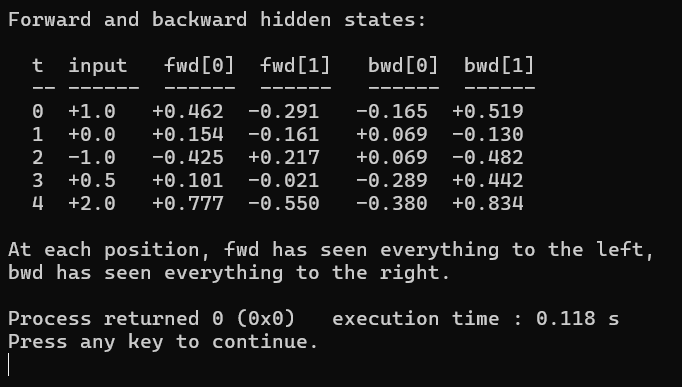
Figure 17-2 has the forward and backward hidden states at every position. Read the table one row at a time and check what each column actually knows. At t=0 the forward state is [+0.462, −0.291] and it has seen exactly one input, the +1.0 at position 0, because there is no history before the start. The backward state at that same position is [−0.165, +0.519] and it has seen every input in the sequence, since it began at t=4 and worked down. The two halves of that row are built from completely different evidence despite sitting side by side.
Position 4 is the mirror image. The forward state has reached [+0.777, −0.550] having consumed all five inputs, while the backward state is [−0.380, +0.834] having consumed only the single +2.0 at that position. So the amount of context each direction carries varies across the sequence, running from nothing to everything for the forward pass and from everything to nothing for the backward pass, and at every position the two sum to the whole.
The middle rows are where the arrangement earns its cost. At t=2 the forward state has absorbed the inputs at 0, 1 and 2 while the backward state has absorbed 4, 3 and 2, so position 2 is the only element covered by both. Neither direction alone has the full picture at any interior position, and both together always do. Notice also that neither state is a simple function of the input at its own position, since the forward state at t=2 is [−0.425, +0.217] and goes negative while the input there is −1.0, whereas the backward state at the same position is [+0.069, −0.482] and disagrees on both components. They are reading the same sequence and reaching different conclusions, which is the point of keeping both.
17.4 Combining the Two Directions
Two hidden states per position is awkward for whatever comes next, so they need joining into a single representation. Concatenation is the standard answer, meaning the two vectors are simply laid end to end into one vector of twice the length, and it is standard precisely because it throws nothing away.
/* 093_Combine.c */
#include <stdio.h>
#include <math.h>

static float my_tanh(float z)
{
    if (z < -20) return -1;
    float e = expf(-2 * z);
    return (1 - e) / (1 + e);
}

#define N_HID 2
#define SEQ_LEN 5
#define N_COMBINED (2 * N_HID)  /* forward + backward */

static void rnn_step(const float w_x[N_HID],
                     const float w_h[N_HID][N_HID],
                     const float b[N_HID], float x,
                     const float h_old[N_HID],
                     float h_new[N_HID])
{
    int i, j;
    for (i = 0; i < N_HID; i++) {
        float z = b[i] + w_x[i] * x;
        for (j = 0; j < N_HID; j++)
            z += w_h[i][j] * h_old[j];
        h_new[i] = my_tanh(z);
    }
}

int main(void)
{
    float seq[SEQ_LEN] = { 1.0f, 0.0f, -1.0f,
        0.5f, 2.0f };

    float fw_x[N_HID] = { 0.5f, -0.3f };
    float fw_h[N_HID][N_HID] =
        {{ 0.4f, 0.1f }, { -0.1f, 0.4f }};
    float fw_b[N_HID] = { 0, 0 };

    float bw_x[N_HID] = { -0.2f, 0.6f };
    float bw_h[N_HID][N_HID] =
        {{ 0.3f, -0.1f }, { 0.2f, 0.3f }};
    float bw_b[N_HID] = { 0, 0 };

    float h_fwd[SEQ_LEN][N_HID], h_bwd[SEQ_LEN][N_HID];
    float combined[SEQ_LEN][N_COMBINED];
    int t, i;

    /* Forward pass */
    for (t = 0; t < SEQ_LEN; t++)
        rnn_step(fw_x, fw_h, fw_b, seq[t],
                 t == 0 ? (float[]){0, 0} : h_fwd[t-1],
                 h_fwd[t]);

    /* Backward pass */
    for (t = SEQ_LEN - 1; t >= 0; t--)
        rnn_step(bw_x, bw_h, bw_b, seq[t],
                 t == SEQ_LEN-1
                     ? (float[]){0, 0} : h_bwd[t+1],
                 h_bwd[t]);

    /* Concatenate */
    for (t = 0; t < SEQ_LEN; t++) {
        for (i = 0; i < N_HID; i++) {
            combined[t][i] = h_fwd[t][i];
            combined[t][N_HID + i] = h_bwd[t][i];
        }
    }

    printf("Combined bidirectional "
           "representations:\n\n");
    printf("  t  input   combined[0..3]\n");
    printf("  -- ------  ------------------------"
           "--------\n");
    for (t = 0; t < SEQ_LEN; t++) {
        printf("  %d  %+4.1f   [%+.3f, %+.3f | "
               "%+.3f, %+.3f]\n",
               t, seq[t],
               combined[t][0], combined[t][1],
               combined[t][2], combined[t][3]);
    }

    printf("\nThe | separates forward (left) from "
           "backward (right).\n");
    printf("Each position has a %d-dimensional "
           "representation\n", N_COMBINED);
    printf("that encodes context from both "
           "directions.\n");

    printf("\nThe output layer takes the combined "
           "vector.\n");
    printf("  y_t = W_out * combined_t + b_out\n");
    printf("  W_out has %d columns instead of %d.\n",
           N_COMBINED, N_HID);

    return 0;
}
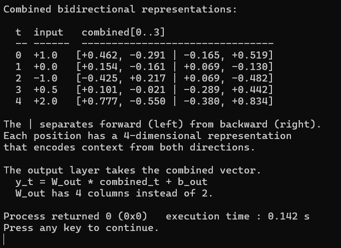
Figure 17-3 lays the two directions end to end into one representation per position. The output puts a vertical bar where the join happens, so each row reads as forward pair, bar, backward pair. At t=0 the combined vector is [+0.462, −0.291 | −0.165, +0.519], and those are exactly the four numbers from the previous section with no arithmetic performed on them at all. Concatenation is a bookkeeping operation rather than a computation, which is why it preserves everything.
The first half of every combined vector encodes left context and the second half encodes right context, and crucially they stay separable. A downstream weight matrix has one column per element, so it can learn to weight left context differently from right context, and it can learn to weight them differently for each class it predicts. That freedom disappears the moment you combine the directions arithmetically. Adding the two vectors instead of concatenating them would keep the dimension at two rather than four, which sounds like a saving until you notice that +0.462 and −0.165 would collapse to +0.297 and nothing downstream could ever recover which direction contributed what.
The cost is dimension. Every position now carries a vector twice as wide, so the output layer that reads it needs twice as many weights per class, which the closing lines of the program spell out as W_out having four columns where a unidirectional model would need two. That doubling is on top of the doubling in the recurrent weights themselves, since there are two complete cells rather than one.
17.5 Bidirectional Output Layer
A combined representation is only useful once something reads it, so this step attaches a classifier that produces a tag for every position. That is the standard shape for sequence labelling, where the input and the output have the same length and each element of the output depends on the whole input.
/* 094_Output.c */
#include <stdio.h>
#include <math.h>
#include <float.h>

static float my_tanh(float z)
{
    if (z < -20) return -1;
    float e = expf(-2 * z);
    return (1 - e) / (1 + e);
}

#define N_HID 3
#define SEQ_LEN 6
#define N_COMBINED (2 * N_HID)
#define N_CLASSES 5

static void rnn_step(const float w_x[N_HID],
                     const float w_h[N_HID][N_HID],
                     const float b[N_HID], float x,
                     const float h_old[N_HID],
                     float h_new[N_HID])
{
    int i, j;
    for (i = 0; i < N_HID; i++) {
        float z = b[i] + w_x[i] * x;
        for (j = 0; j < N_HID; j++)
            z += w_h[i][j] * h_old[j];
        h_new[i] = my_tanh(z);
    }
}

static void softmax(float *x, int n)
{
    float mx = -FLT_MAX, s = 0;
    int i;
    for (i = 0; i < n; i++) if (x[i] > mx) mx = x[i];
    for (i = 0; i < n; i++) {
        x[i] = expf(x[i] - mx);
        s += x[i];
    }
    for (i = 0; i < n; i++) x[i] /= s;
}

int main(void)
{
    /* Simulated word embeddings for a 6-word
       sentence */
    float seq[SEQ_LEN] =
        { 0.2f, -0.5f, 0.8f, -0.1f, 0.6f, -0.3f };
    const char *words[] = { "The", "old", "man",
                            "sat", "on", "chair" };
    const char *labels[] = { "DET", "ADJ", "NOUN",
                             "VERB", "PREP", "NOUN" };

    /* Forward and backward RNN weights */
    float fw_x[N_HID] = {0.5f, -0.3f, 0.2f};
    float fw_h[N_HID][N_HID] = {{0.3f, 0.1f, 0},
                               {0, 0.3f, 0.1f},
                               {0.1f, 0, 0.3f}};
    float fw_b[N_HID] = {0, 0, 0};
    float bw_x[N_HID] = {-0.2f, 0.4f, 0.1f};
    float bw_h[N_HID][N_HID] = {{0.3f, 0, -0.1f},
                               {0.1f, 0.3f, 0},
                               {0, 0.1f, 0.3f}};
    float bw_b[N_HID] = {0, 0, 0};

    /* Output weights: N_CLASSES x N_COMBINED */
    /* One row per tag, DET ADJ NOUN VERB PREP */
    float W_out[N_CLASSES][N_COMBINED] = {
        { 1.0f, 0.2f, -0.3f, 0.5f, -0.1f, 0.4f },
        { -0.5f, 0.8f, 0.1f, -0.2f, 0.6f, -0.3f },
        { 0.2f, -0.4f, 0.7f, 0.1f, -0.3f, 0.5f },
        { -0.3f, 0.5f, -0.2f, 0.7f, 0.2f, -0.4f },
        { 0.4f, 0.1f, -0.6f, -0.3f, 0.5f, 0.2f },
    };
    float b_out[N_CLASSES] = { 0, 0, 0, 0, 0 };

    float h_fwd[SEQ_LEN][N_HID], h_bwd[SEQ_LEN][N_HID];
    int t, i, j;

    /* Forward pass */
    for (t = 0; t < SEQ_LEN; t++)
        rnn_step(fw_x, fw_h, fw_b, seq[t],
                 t == 0 ? (float[])
                 {
                     0, 0, 0
                 }
                        : h_fwd[t-1],
                 h_fwd[t]);

    /* Backward pass */
    for (t = SEQ_LEN - 1; t >= 0; t--)
        rnn_step(bw_x, bw_h, bw_b, seq[t],
                 t == SEQ_LEN-1
                     ? (float[]){0, 0, 0} : h_bwd[t+1],
                 h_bwd[t]);

    /* Classify each position */
    printf("Bidirectional RNN for sequence "
           "labeling:\n\n");
    printf("  word    gold   "
           "DET   ADJ   NOUN  VERB  PREP   pred\n");
    printf("  ------  -----  ----  ----  ----  "
           "----  ----   ----\n");

    for (t = 0; t < SEQ_LEN; t++) {
        /* Concatenate */
        float combined[N_COMBINED];
        for (i = 0; i < N_HID; i++) {
            combined[i] = h_fwd[t][i];
            combined[N_HID + i] = h_bwd[t][i];
        }

        /* Linear + softmax */
        float logits[N_CLASSES];
        for (i = 0; i < N_CLASSES; i++) {
            logits[i] = b_out[i];
            for (j = 0; j < N_COMBINED; j++)
                logits[i] += W_out[i][j] * combined[j];
        }
        softmax(logits, N_CLASSES);

        /* Find predicted class */
        int pred = 0;
        for (i = 1; i < N_CLASSES; i++)
            if (logits[i] > logits[pred]) pred = i;

        const char *class_names[] = { "DET", "ADJ",
                                      "NOUN", "VERB",
                                      "PREP" };
        printf("  %-6s  %-5s  %.2f  %.2f  %.2f  "
               "%.2f  %.2f   %s\n",
               words[t], labels[t],
               logits[0], logits[1], logits[2],
               logits[3], logits[4],
               class_names[pred]);
    }

    printf("\nWeights are random, so predictions "
           "are wrong.\n");
    printf("With training, the bidirectional "
           "context would let\n");
    printf("the model correctly tag each word.\n");

    return 0;
}
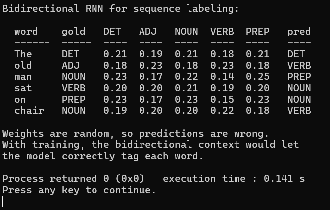
Figure 17-4 reads the combined vector at each word and picks among five tags. The sentence is “The old man sat on chair” and the gold tags run DET, ADJ, NOUN, VERB, PREP, NOUN, so the classifier has five distinct tags to choose between and produces a probability for each at every position. Read across any row and the five numbers sum to 1, which is the softmax doing its job, and read down any column and you can see the model has no idea what it is doing.
That is expected, and saying so plainly beats skating past it. The weights here are hand written constants rather than trained parameters, so the probabilities sit between 0.14 and 0.25 across the board, barely distinguishable from the 0.20 that five equally likely classes would give. The model tags The correctly as DET, which is luck rather than skill, and then gets old wrong as VERB and man wrong as PREP. What the listing demonstrates is the wiring rather than the accuracy, and the wiring is correct in that every one of the six positions produced a distribution over all five tags from a representation built out of both directions.
Look at the shape of the output layer while it is in front of you. W_out has one row per tag and one column per element of the combined vector, so five rows of six columns here, where a unidirectional model of the same hidden size would need five rows of three. Every additional tag costs six weights rather than three, and that ratio holds however many tags the tag set contains. This is the concrete price of the doubling described in the previous section, and in exchange the decision at position 2 can draw on the word at position 5.
17.6 When Bidirectional Helps and Hurts
Everything above carries an unstated requirement, and it is a hard constraint rather than a preference. The backward pass starts at the last element of the sequence, so it cannot begin until the last element exists, which means a bidirectional model produces no output at all until the entire input has arrived. That single fact divides every sequence task into two groups, and the dividing line is availability rather than difficulty.
On one side sit the tasks where the whole input is already in memory before processing starts. Part-of-speech tagging and named entity recognition both label text that is sitting in a file. Sentiment classification over a complete review has the review. Speech recognition on a recorded utterance has the recording. The encoder half of a sequence to sequence model, which Chapter 18 builds, reads the entire source sentence before the decoder emits a single word. Nothing is lost by waiting in any of these, because there is nothing to wait for.
On the other side sit the tasks that must emit output while input is still arriving, and for these bidirectionality is not merely inadvisable, it is impossible. A language model predicting the next word cannot see the next word, which is the definition of the task rather than a limitation of the architecture. Real-time speech has to produce text as audio streams in. Robot control has to act on the sensor reading it has rather than the one arriving next second. Autoregressive generation manufactures its own future one token at a time, so a backward pass would need to consume text the model has not written yet. In every case the backward pass would require information that does not exist.
There is a second cost, smaller but worth counting. A bidirectional model runs two complete cells rather than one, so its recurrent parameters double, and the classifier reading the concatenated representation sees an input of twice the width.
| Unidirectional GRU | Bidirectional GRU | |
|---|---|---|
| Recurrent parameters | 18,624 | 37,248 |
| Output layer input | 64 | 128 |
Those figures use a hidden size of 64 and an input size of 32, and the 18,624 is the same number Chapter 16 arrived at for a single GRU. So bidirectionality doubles the recurrent cost and doubles the classifier input, and in exchange it supplies context that a unidirectional model cannot obtain at any price. That is a different kind of bargain from the GRU against LSTM choice in Chapter 16, where both options could in principle solve the same task and one was merely cheaper.
The same split reappears at much larger scale in Chapter 24 and beyond. BERT is an encoder that attends in both directions, which makes it strong at labelling and classification and incapable of generation. GPT is a decoder that attends only to the past, which makes generation possible. Neither is the better architecture in the abstract. The choice between them is exactly the choice described here, made once at the top of the design rather than layer by layer.
17.7 Bidirectional with GRU Cells
Nothing in the wrapper depends on what kind of cell sits inside it, which is worth demonstrating rather than asserting. Swapping the basic RNN cells for the GRU cells from Chapter 16 changes the cell function and leaves the surrounding structure untouched, giving the BiGRU that carried sequence labelling for most of the decade before transformers.
/* 095_Bigru.c */
#include <stdio.h>
#include <math.h>
#include <stdlib.h>

static float sigmoid(float z)
{
    return 1.0f / (1.0f + expf(-z));
}
static float my_tanh(float z)
{
    if (z < -20) return -1;
    float e = expf(-2 * z);
    return (1 - e) / (1 + e);
}
static float randf(void)
{
    return (float)rand() / RAND_MAX;
}

#define N 3
#define SEQ_LEN 8

typedef struct {
    float W_z[N], U_z[N][N], b_z[N];
    float W_r[N], U_r[N][N], b_r[N];
    float W_s[N], U_s[N][N], b_s[N];
}
GRUCell;

static void gru_step(const GRUCell *g, float x,
                      const float hp[N], float hn[N])
{
    int i, j;
    for (i = 0; i < N; i++) {
        float zz = g->b_z[i] + g->W_z[i] * x;
        float zr = g->b_r[i] + g->W_r[i] * x;
        for (j = 0; j < N; j++) {
            zz += g->U_z[i][j] * hp[j];
            zr += g->U_r[i][j] * hp[j];
        }
        float z = sigmoid(zz), r = sigmoid(zr);
        float zs = g->b_s[i] + g->W_s[i] * x;
        for (j = 0; j < N; j++)
            zs += g->U_s[i][j] * (r * hp[j]);
        float s = my_tanh(zs);
        hn[i] = z * hp[i] + (1 - z) * s;
    }
}

static void gru_init(GRUCell *g)
{
    int i, j;
    for (i = 0; i < N; i++) {
        g->W_z[i] = randf()*0.4f-0.2f;
        g->b_z[i] = 0;
        g->W_r[i] = randf()*0.4f-0.2f;
        g->b_r[i] = 0;
        g->W_s[i] = randf()*0.4f-0.2f;
        g->b_s[i] = 0;
        for (j = 0; j < N; j++) {
            g->U_z[i][j] = randf()*0.2f-0.1f;
            g->U_r[i][j] = randf()*0.2f-0.1f;
            g->U_s[i][j] = randf()*0.2f-0.1f;
        }
    }
}

int main(void)
{
    GRUCell fwd_cell, bwd_cell;
    float seq[SEQ_LEN] = { 0.5f, -0.2f, 0.8f, 0.1f,
                           -0.5f, 0.3f, 0.9f, -0.1f };

    float h_fwd[SEQ_LEN][N], h_bwd[SEQ_LEN][N];
    float h_zero[N] = {0};
    int t, i;

    srand(42);
    gru_init(&fwd_cell);
    gru_init(&bwd_cell);

    /* Forward GRU */
    for (t = 0; t < SEQ_LEN; t++)
        gru_step(&fwd_cell, seq[t],
                 t == 0 ? h_zero : h_fwd[t-1],
                 h_fwd[t]);

    /* Backward GRU */
    for (t = SEQ_LEN - 1; t >= 0; t--)
        gru_step(&bwd_cell, seq[t],
                 t == SEQ_LEN-1 ? h_zero : h_bwd[t+1],
                 h_bwd[t]);

    printf("Bidirectional GRU (BiGRU):\n\n");
    printf("  t  input   fwd             bwd     "
           "        |fwd|  |bwd|\n");
    printf("  -- ------  --------------- ---------"
           "------ ------ ------\n");

    for (t = 0; t < SEQ_LEN; t++) {
        float nf = 0, nb = 0;
        for (i = 0; i < N; i++) {
            nf += h_fwd[t][i] * h_fwd[t][i];
            nb += h_bwd[t][i] * h_bwd[t][i];
        }
        printf("  %d  %+4.1f   [%+.2f,%+.2f,%+.2f] "
               "[%+.2f,%+.2f,%+.2f] %.3f  %.3f\n",
               t, seq[t],
               h_fwd[t][0], h_fwd[t][1], h_fwd[t][2],
               h_bwd[t][0], h_bwd[t][1], h_bwd[t][2],
               sqrtf(nf), sqrtf(nb));
    }

    printf("\nEach position has %d forward plus %d "
           "backward = %d combined.\n", N, N, 2*N);
    printf("The GRU gates handle long-range "
           "dependencies.\n");
    printf("The bidirectional structure handles "
           "both directions.\n");
    printf("Together they give long-range, "
           "full-context representations.\n");

    return 0;
}
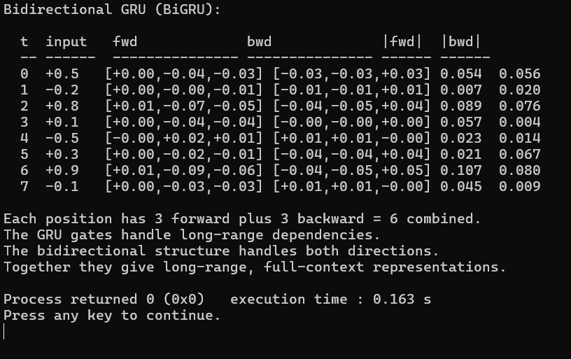
Figure 17-5 runs a BiGRU and reports the norm of each direction per position. Two extra columns hold the norm of each direction’s hidden state, which is the fastest way to see how unevenly the two contribute. At t=0 they sit at 0.054 and 0.056, near enough identical, and at t=2 they are 0.089 and 0.076, so at those positions both directions are carrying comparable signal. Then look at t=3, where the forward norm is 0.057 and the backward norm is 0.004, a factor of fourteen apart. A model reading the concatenated vector at that position is effectively working from one direction only, and nothing in the representation tells it so.
The table explains its own asymmetry if you read the neighboring rows. The backward state at t=3 is built from the input at position 3, which is only +0.1, and from the backward state at t=4, whose norm is already down to 0.014. A small input arriving on top of an almost empty state produces an almost empty state. The forward state at the same position is built from that same small +0.1 input but arrives carrying the forward state from t=2, whose norm of 0.089 is the largest in its column because it was driven by the +0.8 input there. Roughly half of that survives the GRU’s per step decay and lands at t=3.
Position 7 shows the same pattern less extremely, with 0.045 forward against 0.009 backward, and for the same reason, since the backward pass has barely started there while the forward pass has consumed the whole sequence. The general point is that the two directions see different subsequences and there is no reason for those subsequences to carry equal information, so an uneven split is the normal case rather than the exception. A trained model learns to weight the two halves differently per position, which it can only do because concatenation kept them separable.
The values themselves are small, running between 0.004 and 0.107, for the same reason every untrained example in Chapters 15 and 16 produced small values. The gates start near their neutral positions, the weights are random and tiny, and nothing has learned to respond strongly to anything yet. What matters here is that the structure runs end to end with a gated cell in place of a plain one, and that the per position representation is six numbers built from three forward and three backward, which the closing line confirms.
17.8 Key Takeaways
A bidirectional RNN runs two independent recurrent networks over the same sequence, one left to right and one right to left. They share no parameters, so the backward network is a separate model rather than the forward one reversed.
At every position the forward state carries everything to the left and the backward state carries everything to the right. We saw the extremes, where position 0 has one input of forward context and the whole sequence of backward context, and position 4 has the reverse.
The two states are concatenated rather than added, which doubles the representation width and keeps the directions separable. Adding them would hold the width constant and destroy the ability of any downstream layer to weight left and right context differently.
The output layer reads the combined vector, so it needs twice as many weights per class. We used five tags over a six wide combined vector, where a unidirectional model of the same hidden size would have needed five rows of three.
Bidirectional models require the entire sequence before producing any output, because the backward pass starts at the last element. This rules them out for language modeling, real-time speech, robot control and autoregressive generation, no matter how well they would otherwise perform.
The wrapper works over any recurrent cell. We swapped GRU cells in without touching the surrounding structure, and BiLSTM and BiGRU are the two common choices in practice.
Parameters double, since two complete cells run instead of one. A unidirectional GRU at hidden 64 and input 32 costs 18,624 and the bidirectional version costs 37,248, with the classifier input widening from 64 to 128 on top.
The two directions rarely contribute equally at a given position. The BiGRU measured a forward norm of 0.057 against a backward norm of 0.004 at one position, a factor of fourteen, because the two passes see different subsequences and those subsequences carry different amounts of information.
BERT and GPT are the same split at transformer scale. BERT attends both ways and cannot generate, GPT attends only backward and can, and the choice turns on whether the task can wait for the whole input.
17.9 Exercises
Run 093_Combine.c and compare the combined representation at position 0 and position 4. Position 0 has full forward context but only backward context from the last position. Position 4 is the reverse. Is this a problem?
Instead of concatenation, try addition, so combined[i] = fwd[i] + bwd[i]. The representation stays the same size. What information is lost?
Build a bidirectional LSTM using the LSTM cell from Chapter 15. Compare the output representations to the BiGRU.
Implement a simple sequence labeling task, where given a sequence of 0s and 1s, label each position as “inside a run of 1s” or “not.” Train a unidirectional GRU and a BiGRU. Which one is more accurate at the boundaries of runs?
How would you use a bidirectional RNN for sentence-level classification (e.g., sentiment)? You need a single output, not one per position. What do you do with the per-position representations?
Stack two BiGRU layers. The second layer takes the concatenated output of the first layer as input. What is the total representation dimension? How many parameters does this add?