Normalization Deep Dive
LayerNorm, RMSNorm, pre-norm vs post-norm
23.1 What You Will Learn
A transformer is a stack of layers that each add something to their input, and the trouble with adding is that it accumulates. If every layer grows the magnitude of the activations even slightly, then twenty four layers later the numbers arriving at the output are nothing like the numbers that went in. Large activations produce large gradients and unstable updates, small activations produce gradients that vanish, and neither failure announces itself until training has already gone wrong.
Normalization holds the scale steady. This chapter builds Layer Normalization, which subtracts the mean and divides by the standard deviation, and then RMS Normalization, which drops the mean subtraction and turns out to work about as well for a third less arithmetic.
The more interesting question is where to put them, and we answer that later on with a measurement rather than an argument. Putting the normalization before each sublayer instead of after it changes how much gradient survives a deep stack, and the difference is large enough to decide whether a hundred layer model trains at all. The chapter finishes with the backward pass, verified numerically against finite differences.
23.2 The Problem
Chapter 24 builds the residual connection properly, but the shape of it matters here. Each transformer layer computes something from its input and adds the result back, so the value flowing through the stack is a running sum rather than a fresh computation. Sums drift. A layer that multiplies the magnitude by 1.1 looks harmless, and twenty four of them multiply it by roughly ten.
Batch Normalization, which handles this in convolutional networks, normalizes each feature across the examples in a batch. That assumption breaks for sequences in two ways. Different positions in a sentence have genuinely different statistics, so pooling them is the wrong average, and language models often train with batches small enough that the batch statistics are noise.
Layer Normalization takes the perpendicular slice. It normalizes across the features of one vector, so every position of every example is handled on its own and the batch size never enters the calculation. That independence is why it took over for sequence models and why it survived into transformers unchanged.
23.3 The Mean and Variance
Every normalization scheme starts by measuring what it is about to correct, so the first program computes the mean and variance of two vectors chosen to be as different in scale as possible.
/* 120_Stats.c */
#include <stdio.h>
#include <math.h>

#define DIM 6

static void compute_stats(const float *x, int n,
                          float *mean, float *var)
{
    int i;
    double sum = 0, sum_sq = 0;

    for (i = 0; i < n; i++)
        sum += x[i];
    *mean = (float)(sum / n);

    for (i = 0; i < n; i++) {
        float d = x[i] - *mean;
        sum_sq += d * d;
    }
    *var = (float)(sum_sq / n);
}

int main(void)
{
    /* Two vectors with very different scales */
    float a[DIM] = { 100.0f, 102.0f, 98.0f,
                     101.0f, 99.0f, 103.0f };
    float b[DIM] = { 0.001f, 0.003f, -0.001f,
                     0.002f, 0.000f, 0.004f };
    float mean, var;

    compute_stats(a, DIM, &mean, &var);
    printf("Vector a: mean=%.2f  var=%.2f  "
           "std=%.2f\n", mean, var, sqrtf(var));

    compute_stats(b, DIM, &mean, &var);
    printf("Vector b: mean=%.4f  var=%.8f  "
           "std=%.6f\n", mean, var, sqrtf(var));

    printf("\nThese two vectors sit at completely "
           "different scales.\n");
    printf("A dense layer receiving both would "
           "struggle, because\n");
    printf("the same weights must span 98 to 103\n");
    printf("AND values from -0.001 to 0.004.\n");
    printf("Normalization brings both to one scale.\n");

    return 0;
}
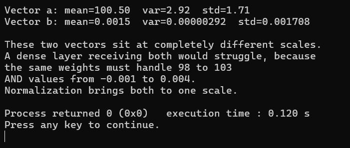
Figure 23-1 has two vectors of the same shape at wildly different scales. Vector a has a mean of 100.50 and a standard deviation of 1.71. Vector b has a mean of 0.0015 and a standard deviation of 0.001708. The two are five orders of magnitude apart in absolute terms.
Look at the ratio inside each vector though, because that is the part that survives normalization. Vector a spans 98 to 103, which is about three standard deviations, and vector b spans −0.001 to 0.004, which is also about three standard deviations. The shape of the two distributions is nearly identical and only the scale differs, which is exactly the situation normalization exists for.
Now picture a dense layer receiving both. Weights large enough to produce a useful response to vector b would produce enormous outputs from vector a, and weights tuned for a would treat b as zero. There is no single setting that handles both, and no amount of training finds one, because the problem is in the input rather than in the weights. Rescale both to the same range and one set of weights serves both.
23.4 Layer Normalization
LayerNorm centers the vector and divides out its spread, then hands the result to two learned parameters that can scale and shift it again.
The gamma and beta exist so the network is not forced to accept zero mean and unit variance if that is not what it wants. Setting gamma to the original standard deviation and beta to the original mean would undo the normalization entirely, and the fact that the network can do that but usually does not is evidence the normalization is helping.
The epsilon guards the division. A vector whose components are all equal has zero variance, and without epsilon the division would produce infinities, which exercise 1 asks you to try.
/* 121_Layernorm.c */
#include <stdio.h>
#include <math.h>

#define DIM 6

typedef struct {
    float gamma[DIM];  /* learned scale */
    float beta[DIM];   /* learned shift */
}
LayerNorm;

static void layernorm_init(LayerNorm *ln, int dim)
{
    int i;
    for (i = 0; i < dim; i++) {
        /* start at 1, an identity scale */
        ln->gamma[i] = 1.0f;
        /* start at 0 (no shift) */
        ln->beta[i] = 0.0f;
    }
}

static void layernorm_forward(const LayerNorm *ln,
                               const float *x,
                               float *out, int dim,
                               float *mean_out,
                               float *std_inv_out)
{
    int i;
    double sum = 0;
    float eps = 1e-5f;

    /* Compute mean */
    for (i = 0; i < dim; i++) sum += x[i];
    float mean = (float)(sum / dim);

    /* Compute variance */
    double var_sum = 0;
    for (i = 0; i < dim; i++) {
        float d = x[i] - mean;
        var_sum += d * d;
    }
    float var = (float)(var_sum / dim);
    float std_inv = 1.0f / sqrtf(var + eps);

    /* Normalize and apply gamma/beta */
    for (i = 0; i < dim; i++)
        out[i] = ln->gamma[i] * (x[i] - mean)
                 * std_inv + ln->beta[i];

    /* Save for backward pass */
    *mean_out = mean;
    *std_inv_out = std_inv;
}

int main(void)
{
    LayerNorm ln;
    layernorm_init(&ln, DIM);

    float x[DIM] = { 100.0f, 102.0f, 98.0f,
                     101.0f, 99.0f, 103.0f };
    float out[DIM];
    float mean, std_inv;
    int i;

    printf("Before LayerNorm:\n  [");
    for (i = 0; i < DIM; i++)
        printf("%.1f%s", x[i], i<DIM-1?", ":"");
    printf("]\n");

    layernorm_forward(&ln, x, out, DIM,
        &mean, &std_inv);

    printf("\nAfter LayerNorm:\n  [");
    for (i = 0; i < DIM; i++)
        printf("%+.4f%s", out[i], i<DIM-1?", ":"");
    printf("]\n");

    /* Verify zero mean and unit variance */
    double out_sum = 0, out_var = 0;
    for (i = 0; i < DIM; i++) out_sum += out[i];
    float out_mean = (float)(out_sum / DIM);
    for (i = 0; i < DIM; i++) {
        float d = out[i] - out_mean;
        out_var += d * d;
    }
    out_var /= DIM;

    printf("\n  Output mean: %.6f, expect ~0\n",
           out_mean);
    printf("  Output var:  %.6f, expect ~1\n",
           (float)out_var);
    printf("\n  mean=%.2f  std_inv=%.4f, saved for "
           "backward\n", mean, std_inv);

    return 0;
}
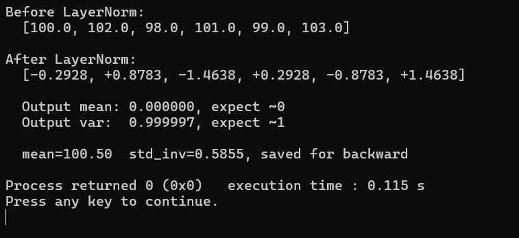
Figure 23-2 brings that vector to zero mean and unit variance. The input runs from 98 to 103 and the output runs from −1.4638 to +1.4638. The program checks its own work and reports an output mean of 0.000000 and an output variance of 0.999997, which is unit variance to within float precision.
Notice that the shape is preserved exactly. The input’s largest value, 103, is the largest by 2.5 above the mean, and after normalization it is +1.4638, which is 2.5 divided by the standard deviation of 1.71. Nothing has been reordered or distorted, the vector has simply been recentered and rescaled.
The last line stores std_inv, the reciprocal of the standard deviation, and that is not a printing convenience. The backward pass at the end of the chapter needs it, and computing it once during the forward pass is cheaper than recovering it later. KANN does the same thing, keeping std_inv in gtmp between the passes, and its forward operation kad_op_stdnorm is the same subtract and multiply we have written here.
The parameter cost is two floats per dimension, one for gamma and one for beta. Against the attention and feedforward weights of the same layer, which run to hundreds of thousands, that is nothing.
23.5 RMSNorm
RMSNorm asks whether the mean subtraction was earning its keep, and concludes that it was not. It divides by the root mean square and stops there.
No mean, no beta, one pass over the data instead of two. LLaMA and DeepSeek-V3 use it throughout, and the original transformer’s LayerNorm is now the minority choice in new models.
/* 122_Rmsnorm.c */
#include <stdio.h>
#include <math.h>

#define DIM 6

typedef struct {
    float gamma[DIM];
}
RMSNorm;

static void rmsnorm_init(RMSNorm *rn, int dim)
{
    int i;
    for (i = 0; i < dim; i++)
        rn->gamma[i] = 1.0f;
}

static void rmsnorm_forward(const RMSNorm *rn,
                             const float *x,
                             float *out, int dim,
                             float *rms_inv_out)
{
    int i;
    float eps = 1e-5f;

    /* Compute root mean square */
    double sum_sq = 0;
    for (i = 0; i < dim; i++)
        sum_sq += x[i] * x[i];
    float rms = sqrtf((float)(sum_sq / dim) + eps);
    float rms_inv = 1.0f / rms;

    /* Normalize and apply gamma (no beta in RMSNorm) */
    for (i = 0; i < dim; i++)
        out[i] = rn->gamma[i] * x[i] * rms_inv;

    *rms_inv_out = rms_inv;
}

int main(void)
{
    RMSNorm rn;
    rmsnorm_init(&rn, DIM);

    float x[DIM] = { 100.0f, 102.0f, 98.0f,
                     101.0f, 99.0f, 103.0f };
    float out[DIM];
    float rms_inv;
    int i;

    printf("Before RMSNorm:\n  [");
    for (i = 0; i < DIM; i++)
        printf("%.1f%s", x[i], i<DIM-1?", ":"");
    printf("]\n");

    rmsnorm_forward(&rn, x, out, DIM, &rms_inv);

    printf("\nAfter RMSNorm:\n  [");
    for (i = 0; i < DIM; i++)
        printf("%+.4f%s", out[i], i<DIM-1?", ":"");
    printf("]\n");

    /* Verify RMS of output is ~1 */
    double out_rms = 0;
    for (i = 0; i < DIM; i++)
        out_rms += out[i] * out[i];
    out_rms = sqrt(out_rms / DIM);
    printf("\n  Output RMS: %.6f, expect ~1\n",
           out_rms);

    printf("\nRMSNorm vs LayerNorm:\n");
    printf("  LayerNorm subtracts the mean then "
           "divides by std, 2*dim params.\n");
    printf("  RMSNorm divides by RMS only, dim "
           "params, and is faster.\n");
    printf("  DeepSeek-V3 uses RMSNorm throughout.\n");

    return 0;
}
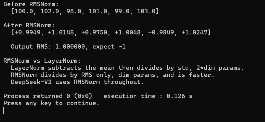
Figure 23-3 runs RMSNorm on the same input. The output runs from +0.9750 to +1.0247 and the reported RMS is 1.000000, so the normalization did what it claims. But compare that against the LayerNorm output for the identical input, which spread from −1.4638 to +1.4638, and something has clearly been lost.
The reason is the input, which we chose earlier to have a large mean. Its RMS is dominated by that mean rather than by the variation around it, so dividing by the RMS leaves every component sitting near 1.0 with the interesting differences squeezed into the third decimal place. LayerNorm removes the mean first and therefore keeps the spread.
That is the honest version of the comparison, and it belongs here rather than after the usual claim that the two are interchangeable. They are interchangeable on zero centered data and they are not on data with a large offset, which the next section measures directly. What makes RMSNorm workable in practice is that activations inside a trained transformer are roughly zero centered already, partly because the layers before them were normalized too.
The saving is real. LayerNorm needs a pass to find the mean, a pass to find the variance, then a subtract and a multiply per element, and it carries two parameter vectors. RMSNorm needs one pass for the sum of squares, one multiply per element, and one parameter vector.
23.6 Comparing the Two
The previous two sections each ran on one input. This one runs both schemes on three inputs chosen to separate them.
/* 123_Compare.c */
#include <stdio.h>
#include <math.h>

#define DIM 5

static void layernorm(const float *x, float *out, int n)
{
    int i;
    double sum = 0;
    float eps = 1e-5f;
    for (i = 0; i < n; i++) sum += x[i];
    float mean = (float)(sum / n);
    double var = 0;
    for (i = 0; i < n; i++) {
        float d = x[i] - mean;
        var += d * d;
    }
    float si = 1.0f / sqrtf((float)(var / n) + eps);
    for (i = 0; i < n; i++) out[i] = (x[i] - mean) * si;
}

static void rmsnorm(const float *x, float *out, int n)
{
    int i;
    double ss = 0;
    float eps = 1e-5f;
    for (i = 0; i < n; i++) ss += x[i] * x[i];
    float ri = 1.0f / sqrtf((float)(ss / n) + eps);
    for (i = 0; i < n; i++) out[i] = x[i] * ri;
}

int main(void)
{
    /* Test case 1: zero-centered data */
    float a[DIM] = { -2.0f, -1.0f, 0.0f, 1.0f, 2.0f };
    /* Test case 2: positive-offset data */
    float b[DIM] = { 8.0f, 9.0f, 10.0f, 11.0f, 12.0f };
    /* Test case 3: mixed signs */
    float c[DIM] = { 3.0f, -1.0f, 0.5f, 2.0f, -0.5f };

    float ln_out[DIM], rms_out[DIM];
    int i;

    struct { const char *name; float
        *data;
        }
        tests[] = {
        { "zero-centered", a },
        { "positive-offset", b },
        { "mixed", c },
    };

    printf("LayerNorm vs RMSNorm comparison:\n\n");

    for (int t = 0; t < 3; t++) {
        float *x = tests[t].data;
        layernorm(x, ln_out, DIM);
        rmsnorm(x, rms_out, DIM);

        printf("  %s: [", tests[t].name);
        for (i = 0; i < DIM; i++)
            printf("%.1f%s", x[i], i<DIM-1?", ":"");
        printf("]\n");

        printf("    LN:  [");
        for (i = 0; i < DIM; i++)
            printf("%+.3f%s", ln_out[i],
                   i<DIM-1?", ":"");
        printf("]\n");

        printf("    RMS: [");
        for (i = 0; i < DIM; i++)
            printf("%+.3f%s", rms_out[i],
                   i<DIM-1?", ":"");
        printf("]\n\n");
    }

    printf("For zero-centered data the two agree.\n");
    printf("For offset data, LN centers first while\n");
    printf("RMS only scales. The gap is usually\n");
    printf("small, because learned "
           "gamma compensates.\n");

    return 0;
}
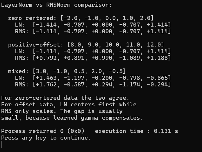
Figure 23-4 sets the two schemes against centered, offset and mixed data. On the zero centered input the two are identical to three decimal places, both giving [−1.414, −0.707, +0.000, +0.707, +1.414]. That is not a coincidence but an identity. When the mean is already zero, subtracting it changes nothing and the variance equals the mean of the squares, so the two formulas reduce to the same expression.
The offset input separates them completely. LayerNorm returns the same [−1.414 to +1.414] spread as before, because subtracting a mean of 10 puts the data back where the first case was. RMSNorm returns [+0.792, +0.891, +0.990, +1.089, +1.188], every value positive and clustered near 1. Both outputs preserve the ordering and the relative gaps, but only one of them uses the available range.
The mixed input, which has a small nonzero mean, lands between the two behaviors as you would expect. LayerNorm gives [+1.463, −1.197, −0.200, +0.798, −0.865] and RMSNorm gives [+1.762, −0.587, +0.294, +1.174, −0.294], different numbers with the same ordering.
Whether the difference matters comes down to gamma. A learned scale can stretch RMSNorm’s compressed output back out, and a learned shift is what LayerNorm’s beta would provide, so a trained network can compensate for most of the gap. What it cannot compensate for is precision lost to the compression, which is why RMSNorm is used in networks where the activations are already centered rather than as a general replacement.
23.7 Pre-Norm and Post-Norm
The original transformer normalized after adding the residual.
Every model of consequence built since normalizes before the sublayer instead, leaving the residual addition as the last thing that happens.
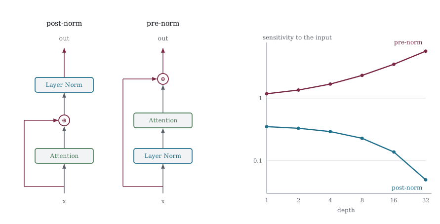
Figure 23-5 puts the two wirings beside the measurement. The blocks are the same blocks in both, and the only change is where the residual addition lands. In post-norm the normalization sits on the residual path, so everything travelling from input to output passes through it. In pre-norm the addition is last, which leaves a route from x to out that touches no normalization at all.
The right panel is what that costs, using the numbers the program prints. Post-norm sensitivity falls from 0.35 at one layer to 0.05 at thirty-two, while pre-norm rises from 1.18 to 5.65. The post-norm curve is the vanishing gradient of Chapter 14 arriving by a different route, and the unnormalized path is exactly what prevents it.
The two look like a formatting choice and are not. This program stacks both arrangements to depths from 1 to 32 and measures how much the output still responds to a change at the input, which is the quantity the first layer’s gradient depends on.
/* 124_Pre_Post.c */
#include <stdio.h>
#include <math.h>

#define DIM 4

static void rmsnorm(const float *x, float *out, int n)
{
    float s = 0;
    int i;
    for (i = 0; i < n; i++) s += x[i] * x[i];
    s = sqrtf(s / n + 1e-6f);
    for (i = 0; i < n; i++) out[i] = x[i] / s;
}

/* A stand-in sublayer. Any fixed function will do,
   what matters is where the norm sits around it. */
static void sublayer(const float *x, float *out, int n)
{
    int i;
    for (i = 0; i < n; i++)
        out[i] = 0.5f * x[i] + 0.1f;
}

/* Run depth layers and return the output */
static void run(const float *x0, int depth, int pre,
                float *out)
{
    float h[DIM], t[DIM], n[DIM];
    int d, i;
    for (i = 0; i < DIM; i++) h[i] = x0[i];
    for (d = 0; d < depth; d++) {
        if (pre) {
            /* x + Sublayer(Norm(x)) */
            rmsnorm(h, n, DIM);
            sublayer(n, t, DIM);
            for (i = 0; i < DIM; i++)
                h[i] = h[i] + t[i];
        }
        else {
            /* Norm(x + Sublayer(x)) */
            sublayer(h, t, DIM);
            for (i = 0; i < DIM; i++)
                t[i] = h[i] + t[i];
            rmsnorm(t, h, DIM);
        }
    }
    for (i = 0; i < DIM; i++) out[i] = h[i];
}

static float norm_of(const float *v, int n)
{
    float s = 0;
    int i;
    for (i = 0; i < n; i++) s += v[i] * v[i];
    return sqrtf(s);
}

/* How much does the output move when input 0 moves?
   This is the gradient the first layer would
   receive. */
static float sensitivity(const float *x0, int depth,
                         int pre)
{
    float a[DIM], b[DIM], xp[DIM], d[DIM];
    float eps = 1e-3f;
    int i;
    for (i = 0; i < DIM; i++) xp[i] = x0[i];
    xp[0] += eps;
    run(x0, depth, pre, a);
    run(xp, depth, pre, b);
    for (i = 0; i < DIM; i++)
        d[i] = (b[i] - a[i]) / eps;
    return norm_of(d, DIM);
}

int main(void)
{
    float x0[DIM] = { 1.0f, 2.0f, 3.0f, 4.0f };
    int depths[] = { 1, 2, 4, 8, 16, 32 };
    float o[DIM];
    int k;

    printf("Post-norm  Norm(x + Sublayer(x))\n");
    printf("Pre-norm   x + Sublayer(Norm(x))\n\n");

    printf("           post-norm         pre-norm\n");
    printf("  depth    |out|   dout/dx   |out|   "
           "dout/dx\n");
    printf("  -----    -----   -------   -----   "
           "-------\n");
    for (k = 0; k < 6; k++) {
        int dpt = depths[k];
        float npost, npre, spost, spre;
        run(x0, dpt, 0, o);
        npost = norm_of(o, DIM);
        run(x0, dpt, 1, o);
        npre = norm_of(o, DIM);
        spost = sensitivity(x0, dpt, 0);
        spre = sensitivity(x0, dpt, 1);
        printf("  %5d  %7.3f  %8.5f %7.3f  %8.3f\n",
               dpt, npost, spost, npre, spre);
    }

    printf("\nThe dout/dx columns are what matter. "
           "They\n");
    printf("say how much the output responds to a\n");
    printf("nudge at the input, the gradient the\n");
    printf("first layer would receive.\n\n");

    printf("Post-norm loses it with depth, since\n");
    printf("every layer divides by the accumulated\n");
    printf("norm and those divisions compound.\n");
    printf("Pre-norm holds, because the residual\n");
    printf("path is a plain addition whose\n");
    printf("derivative is 1 at any depth.\n\n");

    printf("Post-norm: original transformer, 2017.\n");
    printf("Pre-norm:  GPT, LLaMA, DeepSeek-V3.\n");

    return 0;
}
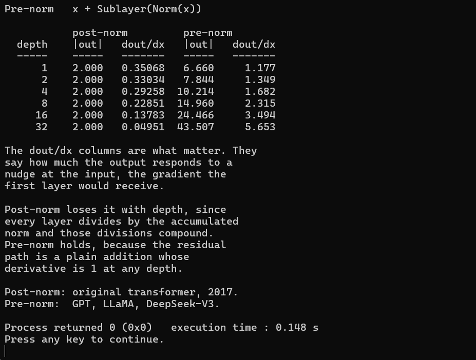
Figure 23-6 tracks sensitivity to the input as the stack gets deeper. The dout/dx columns are the result. Post-norm starts at 0.35068 for a single layer and falls to 0.04951 by 32 layers, losing seven eighths of its sensitivity. Pre-norm starts at 1.177 and rises to 5.653 over the same range. A change at the input of a 32 layer post-norm stack barely reaches the output, and in the backward direction that means the gradient barely reaches the input.
The mechanism is visible in the other pair of columns. Post-norm holds the output norm at exactly 2.000 at every depth, because the last operation in every layer is a normalization that forces it there. Holding the magnitude fixed is precisely what destroys the sensitivity, since each layer must divide by whatever the accumulated residual had grown to, and those divisions compound down the stack. Pre-norm lets the norm grow from 6.660 to 43.507 because nothing at the end of the layer constrains it.
That growth is pre-norm’s own weakness and worth stating rather than hiding. Activations that grow without bound cause their own problems, which is why real pre-norm transformers put one final normalization after the whole stack. What pre-norm buys in exchange is the clean path, since out = x + something means the derivative with respect to x contains an identity term that no depth can attenuate. This is the same trick as the LSTM cell state in Chapter 15, where the gradient travelled along an addition rather than through a multiplication.
Post-norm was the original arrangement and works acceptably at six layers, which is what the 2017 paper used. It stops working somewhere in the low tens. Pre-norm is what allows DeepSeek-V3 to stack 61 layers and train stably.
23.8 The Backward Pass
LayerNorm’s derivative is more involved than most, because every output depends on every input through the shared mean and variance. Changing one component changes the mean, which changes every other normalized value.
The efficient form used by KANN and by this program needs only three quantities, the upstream gradient, the normalized output already computed in the forward pass, and the stored std_inv.
/* 125_Backward.c */
#include <stdio.h>
#include <math.h>

#define DIM 5

static void layernorm_forward(const float *x,
                              float *out,
                               int n,
                                   float *std_inv_out)
{
    int i;
    double sum = 0;
    float eps = 1e-5f;
    for (i = 0; i < n; i++) sum += x[i];
    float mean = (float)(sum / n);
    double var = 0;
    for (i = 0; i < n; i++) {
        float d = x[i] - mean;
        var += d * d;
    }
    float si = 1.0f / sqrtf((float)(var / n) + eps);
    for (i = 0; i < n; i++) out[i] = (x[i] - mean) * si;
    *std_inv_out = si;
}

/* KANN-style backward: efficient closed form */
static void layernorm_backward(const float *upstream,
                                const float *normed,
                                float std_inv,
                                float *grad_in, int n)
{
    int i;
    double sum_g = 0, sum_gx = 0;

    /* Compute two dot products */
    for (i = 0; i < n; i++) {
        sum_g += upstream[i];
        sum_gx += normed[i] * upstream[i];
    }
    float mean_g = (float)(sum_g / n);
    float mean_gx = (float)(sum_gx / n);

    /* grad_in = std_inv * (upstream
         - mean(upstream)
         - normed * mean(normed * upstream)) */
    for (i = 0; i < n; i++)
        grad_in[i] = std_inv * (upstream[i] - mean_g
                     - normed[i] * mean_gx);
}

int main(void)
{
    float x[DIM] = { 1.0f, 3.0f, 2.0f, 5.0f, 4.0f };
    float normed[DIM], grad_in[DIM];
    float std_inv;
    float upstream[DIM] =
        { 0.1f, -0.2f, 0.3f, -0.1f, 0.2f };
    int i;

    layernorm_forward(x, normed, DIM, &std_inv);

    printf("Input:      [");
    for (i = 0; i < DIM; i++)
        printf("%.1f%s", x[i], i<DIM-1?", ":"");
    printf("]\n");
    printf("Normalized: [");
    for (i = 0; i < DIM; i++)
        printf("%+.4f%s", normed[i], i<DIM-1?", ":"");
    printf("]\n");
    printf("Upstream:   [");
    for (i = 0; i < DIM; i++)
        printf("%+.1f%s", upstream[i],
               i<DIM-1?", ":"");
    printf("]\n\n");

    layernorm_backward(upstream, normed, std_inv,
                       grad_in, DIM);

    printf("Gradient:   [");
    for (i = 0; i < DIM; i++)
        printf("%+.4f%s", grad_in[i],
               i<DIM-1?", ":"");
    printf("]\n");

    /* Verify with numerical gradient */
    printf("\nNumerical verification:\n");
    float h = 0.0001f;
    for (i = 0; i < DIM; i++) {
        float x_plus[DIM], x_minus[DIM];
        float out_p[DIM], out_m[DIM], si;
        int j;
        for (j = 0; j < DIM; j++)
            x_plus[j] = x_minus[j] = x[j];
        x_plus[i] += h;
        x_minus[i] -= h;
        layernorm_forward(x_plus, out_p, DIM, &si);
        layernorm_forward(x_minus, out_m, DIM, &si);

        float num_grad = 0;
        for (j = 0; j < DIM; j++)
            num_grad += upstream[j]
                        * (out_p[j] - out_m[j]) / (2*h);

        printf("  dim %d: analytical=%+.4f  "
               "numerical=%+.4f  match=%s\n",
               i, grad_in[i], num_grad,
               fabsf(grad_in[i] - num_grad) < 0.001f
                   ? "yes" : "NO");
    }

    return 0;
}
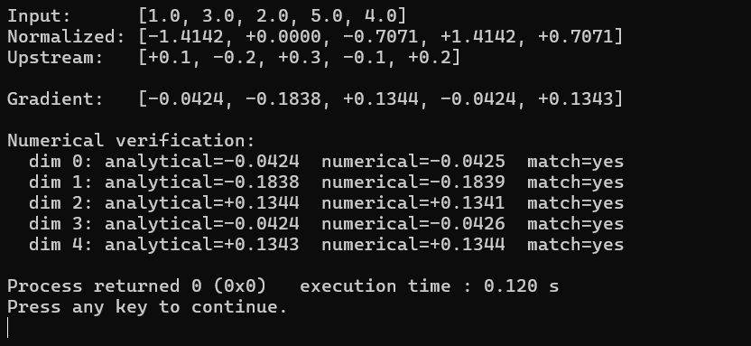
Figure 23-7 checks the backward pass against finite differences. The analytical gradient comes out as [−0.0424, −0.1838, +0.1344, −0.0424, +0.1343], and the verification block recomputes each component by finite differences and compares. All five match, with the largest disagreement being 0.0003 at dimension 2, which is the expected size of error for a central difference with the step used.
That verification is the point of the listing. A backward pass is the easiest thing in a neural network to get subtly wrong, because a wrong gradient still trains, just badly, and nothing crashes. Comparing against finite differences takes a few lines and settles it, which is why exercise 2 asks you to do the same for RMSNorm.
The formula itself is worth reading once slowly. The gradient is std_inv times the upstream gradient, minus the mean of the upstream gradient, minus the normalized output times the mean of the normalized output times the upstream gradient. The two subtracted terms are the corrections for the fact that the mean and the variance both depend on every input. Drop them and the gradient is wrong in a way that still looks plausible.
What it does not need is the original input, or the mean, or the variance. Two dot products and one pass, using only what the forward pass already had reason to keep, which is why KANN stores std_inv in gtmp rather than recomputing anything.
23.9 Key Takeaways
Layer Normalization works across the feature dimension of a single vector, so batch size and sequence position never enter the calculation. Batch Normalization pools across examples, which is the wrong average for sequences.
The formula subtracts the mean, divides by the standard deviation, then applies learned gamma and beta. We measured an output mean of 0.000000 and variance of 0.999997 on a vector that started between 98 and 103.
Epsilon is not decoration. A vector of identical values has zero variance and the division would fail without it.
RMSNorm drops the mean subtraction and the beta parameter, halving the passes over the data and the parameter count.
The two are identical on zero centered data, which we confirmed by getting [−1.414, −0.707, +0.000, +0.707, +1.414] from both. On offset data they diverge, with LayerNorm keeping the full range while RMSNorm compressed the same input to between +0.792 and +1.188.
Pre-norm applies the normalization to the sublayer input and leaves the residual addition last. Post-norm normalizes the sum.
We measured the difference across depth. Post-norm sensitivity fell from 0.35068 at one layer to 0.04951 at 32, while pre-norm rose from 1.177 to 5.653.
Post-norm pins the output norm at 2.000 at every depth, and that pinning is what costs the sensitivity, since each layer divides by the accumulated residual and the divisions compound.
Pre-norm lets the activation norm grow instead, reaching 43.507 by 32 layers, which is why real pre-norm stacks add one final normalization after the last layer.
The backward pass needs the upstream gradient, the normalized output and std_inv, and nothing else. We verified all five components against finite differences, the largest disagreement being 0.0003.
Normalization costs 2 * dim parameters for LayerNorm and dim for RMSNorm, which is negligible beside the attention and feedforward weights in the same layer.
23.10 Exercises
Apply LayerNorm to a vector of all identical values (e.g., [5, 5, 5, 5]). What happens? Why is epsilon important here?
Implement the backward pass for RMSNorm. It is simpler than LayerNorm because there is no mean subtraction. Verify numerically.
Stack 10 dense layers without normalization and measure the output magnitude after each layer. Then add LayerNorm after each layer and compare.
Compare the computation cost by counting the number of multiplications and additions for LayerNorm vs RMSNorm on a vector of size 512. What is the speedup?
Read KANN’s `kad_op_stdnorm` in kautodiff.c. Note how it stores std_inv in `p->gtmp` and uses it in the backward pass. Compare the backward formula to our 125_Backward.c.
DeepSeek-V3 applies “additional RMSNorm layers after the compressed latent vectors” in MLA. Why would you normalize the compressed representation before up-projecting?