The Transformer Block
Attention, feedforward, residual, and normalization in one unit
24.1 What You Will Learn
Everything this book needs for a transformer has now been built separately. Chapter 21 produced multi-head attention, which lets every position in a sequence read every other position and lets several heads do it in parallel along different relationships. Chapter 22 gave positions a representation, so that a mechanism which is otherwise blind to order can tell the first token from the fifth. Chapter 23 supplied the normalization that keeps activations at a workable scale and, more importantly, settled the question of where to put it, measuring a post-norm stack losing seven eighths of its input sensitivity across thirty two layers while a pre-norm stack held on. What remains is to put those pieces in one structure and check that the structure can repeat.
The block has two halves that do genuinely different jobs. Attention is the only place where positions exchange information, so every piece of mixing across the sequence happens there and nowhere else in the block. A feedforward network then processes each position entirely on its own, unable to see any other position, which sounds like a limitation until you notice that it holds most of the parameters and does most of the transforming. Each half is wrapped in a normalization applied to its input and a residual addition applied to its output, in the pre-norm arrangement, and the wrapping is what allows the two halves to be stacked dozens deep without the gradient dying on the way back.
That is the entire architecture of a modern language model. A GPT-style network is this block repeated, twelve times for GPT-2 Small and sixty one times for DeepSeek-V3, with an embedding table in front of the stack and an output head behind it, and nothing else of consequence. By the middle of the chapter there is a working block in C, then we stack four of them and measure whether the representation survives, and we finish by counting what the arrangement costs in real models and why the count never matches the number on the model card.
24.2 The Architecture
Two sublayers run in a fixed order, and each one is written the same way.
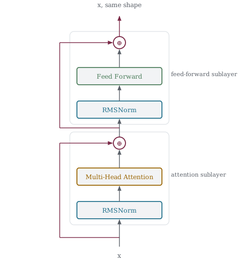
Figure 24-1 is those two lines drawn once. Each sublayer is the same shape, a normalization, the operation itself, and an addition that brings the untouched input back in. The two differ only in what sits in the middle.
Follow the residual line on the left and you can see why blocks stack. It runs from the input to the output without passing through a single normalization, activation or matrix multiply, so a gradient travelling backward has a route home that nothing attenuates. Add a hundred of these and that route is still there.
Read either line from the inside out and the sequence of operations becomes clear. The current value of x is normalized, producing a clean copy at a predictable scale. The sublayer runs on that copy and never sees the raw value. Whatever the sublayer produces is then added back onto the original unnormalized x, so the quantity carried forward through the block, and through every block after it, is a running sum that no normalization ever rescales directly. That last detail is the whole of the pre-norm argument from the last chapter, where the same arrangement held its sensitivity at thirty two layers while post-norm decayed to a twentieth of its starting value, and it should stay in view because everything else in the block depends on that path staying open.
The division of labor between the two sublayers deserves a name, because it explains what depth buys. Attention is the only operation in the block where one position can influence another, so a single block gives the sequence exactly one opportunity to move information from one place to another. The feedforward network then works on each position in isolation, applying the same transformation to every one of them independently, which means it cannot move anything sideways but can reshape whatever attention just delivered. Alternating those two operations is what makes a stack more capable than a single block. After one block, position 5 knows about position 2 directly. After two, it knows about whatever position 2 had already gathered from position 9, and the reach compounds with depth in a way that no single wider block would replicate.
24.3 The Feed-Forward Network
The feedforward network inside a transformer is an ordinary two layer network of the kind Chapter 2 built, with one structural difference that matters more than its simplicity suggests. It is applied to each position separately, with the same weights every time, so a sequence of forty tokens runs the same small network forty times rather than running one large network over the whole sequence. The network widens the representation, applies a nonlinearity, and narrows it back to where it started.
/* 126_Ffn.c */
#include <stdio.h>
#include <math.h>
#include <stdlib.h>

static float randf(void)
{
    return (float)rand() / RAND_MAX;
}

/* GELU approximation */
static float gelu(float x)
{
    float c = 0.7978846f;
    float u = x + 0.044715f * x * x * x;
    return 0.5f * x * (1.0f + tanhf(c * u));
}

#define D_MODEL 6
#define D_FF 12  /* typically 4 * d_model */

typedef struct {
    float W1[D_FF][D_MODEL];   /* up-projection */
    float b1[D_FF];
    float W2[D_MODEL][D_FF];   /* down-projection */
    float b2[D_MODEL];
}
FFN;

static void ffn_init(FFN *f)
{
    int i, j;
    float scale = 0.1f;
    for (i = 0; i < D_FF; i++) {
        f->b1[i] = 0;
        for (j = 0; j < D_MODEL; j++)
            f->W1[i][j] = (randf() * 2 - 1) * scale;
    }
    for (i = 0; i < D_MODEL; i++) {
        f->b2[i] = 0;
        for (j = 0; j < D_FF; j++)
            f->W2[i][j] = (randf() * 2 - 1) * scale;
    }
}

/* FFN forward: up-project, GELU, down-project */
static void ffn_forward(const FFN *f,
                        const float in[D_MODEL],
                         float out[D_MODEL])
{
    float hidden[D_FF];
    int i, j;

    /* Up-project: d_model -> d_ff */
    for (i = 0; i < D_FF; i++) {
        float z = f->b1[i];
        for (j = 0; j < D_MODEL; j++)
            z += f->W1[i][j] * in[j];
        hidden[i] = gelu(z);
    }

    /* Down-project: d_ff -> d_model */
    for (i = 0; i < D_MODEL; i++) {
        float z = f->b2[i];
        for (j = 0; j < D_FF; j++)
            z += f->W2[i][j] * hidden[j];
        out[i] = z;
    }
}

int main(void)
{
    FFN f;
    float in[D_MODEL] = { 0.5f, -0.2f, 0.8f,
                          0.1f, -0.3f, 0.6f };
    float out[D_MODEL];
    int i;

    srand(42);
    ffn_init(&f);
    ffn_forward(&f, in, out);

    printf("Feed-Forward Network, d_model=%d "
           "d_ff=%d\n\n", D_MODEL, D_FF);
    printf("  Input:  [");
    for (i = 0; i < D_MODEL; i++)
        printf("%+.3f%s", in[i],
               i<D_MODEL-1?", ":"");
    printf("]\n  Output: [");
    for (i = 0; i < D_MODEL; i++)
        printf("%+.3f%s", out[i],
               i<D_MODEL-1?", ":"");
    printf("]\n\n");

    int params = D_FF * D_MODEL + D_FF
                 + D_MODEL * D_FF + D_MODEL;
    printf("  Parameters: %d\n", params);
    printf("  Shape: %d -> %d (GELU) -> %d\n",
           D_MODEL, D_FF, D_MODEL);
    printf("  Applied independently "
           "to each position.\n");

    return 0;
}
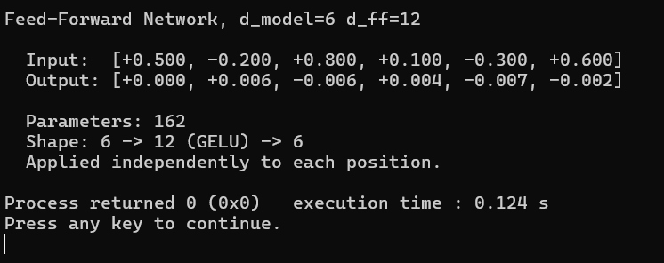
Figure 24-2 widens and narrows one position. The shape line reports 6 to 12 to 6 and the parameter count comes to 162, which breaks down as 72 weights on the way up, 12 biases at the hidden layer, 72 weights on the way down and 6 biases at the output. The widening factor here is 2 so the numbers stay small enough to check by hand, and real models use 4, so a model with a dimension of 512 runs a hidden layer of 2048. The output reads [+0.000, +0.006, −0.006, …] against an input whose components run to 0.8 in magnitude, which is to say the network has produced almost nothing at all. That is the correct behavior for random small weights and not a fault, but it does mean this particular listing demonstrates the shape of the computation rather than anything about what a trained FFN does.
The widening factor is the reason to care, because it decides where a transformer keeps its parameters. Attention in a block costs 4 times d_model squared, covering the query, key, value and output projections, while the feedforward network costs 2 times d_model times d_ff. With the conventional d_ff of four times d_model, that second figure becomes 8 times d_model squared, which is exactly twice what attention costs. Most of the weights in a transformer therefore sit in the half of the block that cannot look sideways at all, which routinely surprises people who assume attention is where a language model keeps what it knows. A useful way to read the FFN is as a lookup, where the first matrix scores the incoming vector against a large set of learned patterns and the second matrix retrieves a weighted combination of learned responses, which makes the hidden dimension a rough measure of how many distinct things a block can recognize.
GELU is the activation here and it is the smooth relative of the ReLU from Chapter 3, passing small negative values through with a slight attenuation rather than clipping them to zero. The original transformer used ReLU, GPT and most models since have used GELU, and DeepSeek-V3 uses SwiGLU, which splits the up-projection into two matrices and gates one with the other. Exercise 6 asks you to build that variant and count what the third matrix costs, and the answer explains why models using it typically shrink d_ff to keep the parameter count level.
24.4 Residual Connection
The residual connection is a single addition and it is the most consequential line in the block, so it gets a listing of its own rather than being buried inside the assembly.
/* 127_Residual.c */
#include <stdio.h>

#define DIM 4

static void residual_add(const float in[DIM],
                         const float sublayer_out[DIM],
                          float out[DIM])
{
    int i;
    for (i = 0; i < DIM; i++)
        out[i] = in[i] + sublayer_out[i];
}

int main(void)
{
    float x[DIM] = { 1.0f, 2.0f, 3.0f, 4.0f };
    float sub[DIM] = { 0.1f, -0.2f, 0.3f, -0.1f };
    float out[DIM];
    int i;

    residual_add(x, sub, out);

    printf("Residual, out = x + sublayer(x)\n\n");
    printf("  Input:     [");
    for (i = 0; i < DIM; i++)
        printf("%.1f%s", x[i], i<DIM-1?", ":"");
    printf("]\n  Sublayer:  [");
    for (i = 0; i < DIM; i++)
        printf("%+.1f%s", sub[i], i<DIM-1?", ":"");
    printf("]\n  Output:    [");
    for (i = 0; i < DIM; i++)
        printf("%.1f%s", out[i], i<DIM-1?", ":"");
    printf("]\n\n");

    printf("  In backprop, d_out/d_x is\n");
    printf("  1 + d_sublayer/d_x\n");
    printf("  Even when d_sublayer/d_x is small,\n");
    printf("  the gradient through the identity\n");
    printf("  path is always 1.\n");
    printf("  Deep transformers train "
           "because of it.\n");

    return 0;
}
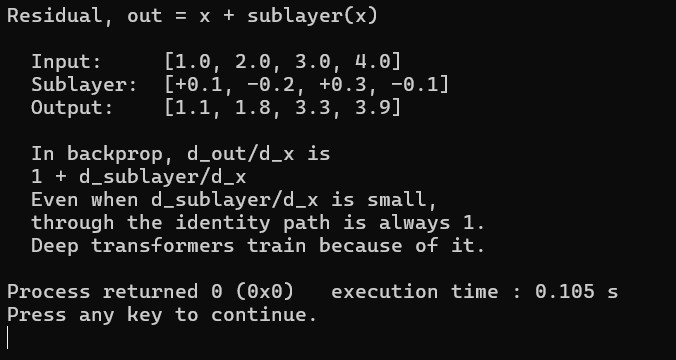
Figure 24-3 has the addition and the identity path it creates. Nothing needs explaining in the forward direction. The input is [1.0, 2.0, 3.0, 4.0], the sublayer produces [+0.1, −0.2, +0.3, −0.1], and adding them component by component gives [1.1, 1.8, 3.3, 3.9]. The backward direction is where the value lies, because differentiating x + f(x) with respect to x gives 1 + f’(x), and that leading 1 does not depend on f in any way. Whatever the sublayer does to the gradient passing through it, however small its derivative happens to be at that point, the identity path delivers the full upstream gradient regardless. A stack of these therefore cannot attenuate a signal the way a stack of matrix multiplications does, because at every layer there is a route to the input that multiplies by exactly one.
This is the third time the book has arrived at the same idea from a different direction, which is worth pausing on. Chapter 15 gave the LSTM a cell state connected across time steps by addition, specifically so that gradient travelling backward through a long sequence would not be multiplied by a weight matrix at every step. Chapter 23 measured the same effect across depth rather than time, finding a pre-norm stack holding a sensitivity of 5.653 at thirty two layers where post-norm had fallen to 0.04951. Here the same structure appears once more inside the block itself. The reason it keeps recurring is not fashion but arithmetic, since addition is the only common operation whose derivative is exactly one, and any architecture that needs a signal to survive many stages ends up using it.
A useful way to think about a deep stack is that the residual path is not a shortcut around the layers but the main channel through them. The value flowing from the first block to the last is a single accumulating vector, and each sublayer reads a normalized copy of it and writes a small correction back. Blocks communicate by leaving things in that shared stream rather than by handing outputs to each other directly, which is why removing the residual does not merely slow training but stops it. Exercise 1 asks you to delete it and watch what happens, first with one block and then with four.
24.5 One Transformer Block
Attention, the feedforward network, two normalizations and two residual additions now go into a single function. The attention here is self-attention, meaning the queries, keys and values are all projected from the same input rather than the queries coming from somewhere else, and the normalization sits before each sublayer in the pre-norm arrangement that Chapter 23 argued for.
/* 128_Block.c */
#include <stdio.h>
#include <math.h>
#include <float.h>
#include <stdlib.h>

static float randf(void)
{
    return (float)rand() / RAND_MAX;
}
static float gelu(float x)
{
    float c = 0.7978846f;
    float u = x + 0.044715f * x * x * x;
    return 0.5f * x * (1.0f + tanhf(c * u));
}

#define SEQ_LEN 4
#define D_MODEL 8
#define N_HEADS 2
#define D_HEAD (D_MODEL / N_HEADS)
#define D_FF (D_MODEL * 4)

/* --- RMSNorm --- */
static void rmsnorm(const float *x, float *out, int n)
{
    int i;
    double ss = 0;
    float eps = 1e-5f;
    for (i = 0; i < n; i++) ss += x[i] * x[i];
    float ri = 1.0f / sqrtf((float)(ss / n) + eps);
    for (i = 0; i < n; i++) out[i] = x[i] * ri;
}

/* --- Multi-Head Self-Attention (simplified) --- */
static float dot(const float *a, const float *b, int n)
{
    float s = 0;
    int i;
    for (i = 0; i < n; i++) s += a[i] * b[i];
    return s;
}

static void softmax(float *x, int n)
{ float mx = -FLT_MAX, s = 0; int i;
  for (i = 0; i < n; i++) if (x[i] > mx) mx = x[i];
    for (i = 0; i < n; i++) {
        x[i] = expf(x[i] - mx);
        s += x[i];
    }
  for (i = 0; i < n; i++) x[i] /= s;
  }

typedef struct {
    float W_Q[N_HEADS][D_HEAD][D_MODEL];
    float W_K[N_HEADS][D_HEAD][D_MODEL];
    float W_V[N_HEADS][D_HEAD][D_MODEL];
    float W_O[D_MODEL][D_MODEL];
}
MHA;

static void mha_forward(const MHA *m,
            const float X[SEQ_LEN][D_MODEL],
                          float out[SEQ_LEN][D_MODEL])
{
    float head_out[N_HEADS][SEQ_LEN][D_HEAD];
    float scale = 1.0f / sqrtf((float)D_HEAD);
    int h, i, j, k, d;

    for (h = 0; h < N_HEADS; h++) {
        for (i = 0; i < SEQ_LEN; i++) {
            /* Project query */
            float q[D_HEAD];
            for (k = 0; k < D_HEAD; k++) {
                q[k] = 0;
                for (d = 0; d < D_MODEL; d++)
                    q[k] += m->W_Q[h][k][d] * X[i][d];
            }
            /* Score every key, then blend values */
            float scores[SEQ_LEN];
            for (j = 0; j < SEQ_LEN; j++) {
                float key[D_HEAD];
                for (k = 0; k < D_HEAD; k++) {
                    key[k] = 0;
                    for (d = 0; d < D_MODEL; d++)
                        key[k] += m
                            ->W_K[h][k][d] * X[j][d];
                }
                scores[j] = dot(q, key, D_HEAD) * scale;
            }
            softmax(scores, SEQ_LEN);
            for (k = 0; k < D_HEAD; k++) {
                head_out[h][i][k] = 0;
                for (j = 0; j < SEQ_LEN; j++) {
                    float val = 0;
                    for (d = 0; d < D_MODEL; d++)
                        val += m
                            ->W_V[h][k][d] * X[j][d];
                    head_out[h][i][k]
                            += scores[j] * val;
                }
            }
        }
    }

    /* Concatenate heads and project with W_O */
    for (i = 0; i < SEQ_LEN; i++) {
        float concat[D_MODEL];
        for (h = 0; h < N_HEADS; h++)
            for (k = 0; k < D_HEAD; k++)
                concat[h * D_HEAD + k] =
                    head_out[h][i][k];
        for (j = 0; j < D_MODEL; j++) {
            out[i][j] = 0;
            for (k = 0; k < D_MODEL; k++)
                out[i][j] += m->W_O[j][k] * concat[k];
        }
    }
}

/* --- Feed-Forward Network --- */
typedef struct {
    float W1[D_FF][D_MODEL];
    float W2[D_MODEL][D_FF];
}
FFN;

static void ffn_forward(const FFN *f,
                        const float in[D_MODEL],
                          float out[D_MODEL])
{
    float hidden[D_FF];
    int i, j;
    for (i = 0; i < D_FF; i++) {
        float z = 0;
        for (j = 0; j < D_MODEL; j++)
            z += f->W1[i][j] * in[j];
        hidden[i] = gelu(z);
    }
    for (i = 0; i < D_MODEL; i++) {
        float z = 0;
        for (j = 0; j < D_FF; j++)
            z += f->W2[i][j] * hidden[j];
        out[i] = z;
    }
}

/* --- Transformer Block --- */
typedef struct {
    MHA attn;
    FFN ffn;
}
TransformerBlock;

static void block_forward(const TransformerBlock *blk,
                            float X[SEQ_LEN][D_MODEL])
{
    float normed[SEQ_LEN][D_MODEL];
    float sublayer[SEQ_LEN][D_MODEL];
    int i, j;

    /* === Sublayer 1: Attention === */
    /* Pre-norm */
    for (i = 0; i < SEQ_LEN; i++)
        rmsnorm(X[i], normed[i], D_MODEL);

    /* Multi-head self-attention */
    mha_forward(&blk->attn, normed, sublayer);

    /* Residual add */
    for (i = 0; i < SEQ_LEN; i++)
        for (j = 0; j < D_MODEL; j++)
            X[i][j] += sublayer[i][j];

    /* === Sublayer 2: FFN === */
    /* Pre-norm */
    for (i = 0; i < SEQ_LEN; i++)
        rmsnorm(X[i], normed[i], D_MODEL);

    /* Feed-forward (per position) */
    for (i = 0; i < SEQ_LEN; i++) {
        float ffn_out[D_MODEL];
        ffn_forward(&blk->ffn, normed[i], ffn_out);
        /* Residual add */
        for (j = 0; j < D_MODEL; j++)
            X[i][j] += ffn_out[j];
    }
}

static void init_random(float *w, int n, float scale)
{
    int i;
    for (i = 0; i < n; i++)
        w[i] = (randf() * 2 - 1) * scale;
}

int main(void)
{
    TransformerBlock blk;
    float X[SEQ_LEN][D_MODEL] = {
        { 1.0f, 0.2f, -0.3f, 0.5f,
          -0.1f, 0.8f, 0.3f, -0.2f },
        { 0.3f, 0.9f, 0.1f, -0.2f,
          0.6f, 0.4f, -0.1f, 0.5f },
        { -0.1f, 0.4f, 0.8f, 0.2f,
          -0.5f, 0.3f, 0.7f, 0.1f },
        { 0.6f, -0.2f, 0.5f, 0.7f,
          0.3f, -0.4f, 0.2f, 0.8f },
    };
    const char *words[] = { "The", "cat",
        "sat", "down" };
    int i, j;

    srand(42);
    init_random((float*)&blk.attn,
                sizeof(MHA)/sizeof(float), 0.1f);
    init_random((float*)&blk.ffn,
                sizeof(FFN)/sizeof(float), 0.1f);

    printf("Transformer block, d_model=%d "
           "heads=%d d_ff=%d\n\n",
           D_MODEL, N_HEADS, D_FF);

    printf("Input:\n");
    for (i = 0; i < SEQ_LEN; i++) {
        printf("  %-5s [", words[i]);
        for (j = 0; j < D_MODEL; j++)
            printf("%+.2f%s", X[i][j],
                j<D_MODEL-1?",":"");
        printf("]\n");
    }

    block_forward(&blk, X);

    printf("\nOutput (after 1 transformer block):\n");
    for (i = 0; i < SEQ_LEN; i++) {
        printf("  %-5s [", words[i]);
        for (j = 0; j < D_MODEL; j++)
            printf("%+.2f%s", X[i][j],
                j<D_MODEL-1?",":"");
        printf("]\n");
    }

    printf("\nOutput shape equals input shape.\n");
    printf("This is critical: blocks "
           "can be stacked.\n");

    /* Parameter count */
    /* W_Q, W_K, W_V and W_O */
    int attn_params = 4 * D_MODEL * D_MODEL;
    /* W1, W2 */
    int ffn_params = 2 * D_MODEL * D_FF;
    /* two RMSNorm gamma vectors */
    int norm_params = 2 * D_MODEL;
    int total = attn_params + ffn_params + norm_params;

    printf("\nParameter count per block:\n");
    printf("  Attention: 4 * %d^2 = %d\n",
           D_MODEL, attn_params);
    printf("  FFN:       2 * %d * %d = %d\n",
           D_MODEL, D_FF, ffn_params);
    printf("  Norms:     2 * %d = %d\n",
           D_MODEL, norm_params);
    printf("  Total:     %d\n", total);

    return 0;
}
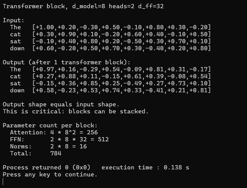
Figure 24-4 runs one complete block, and the input and the output come back the same shape. Set the input and output blocks side by side and they are very nearly the same. The word “The” enters as [+1.00, +0.20, −0.30, +0.50] in its first four components and leaves as [+0.97, +0.16, −0.29, +0.54], with every component having moved only in the second decimal place, and the other three rows behave the same way. A reader expecting a transformer block to transform something could reasonably wonder what happened.
The answer is that this is correct behavior at initialization and that it is a property worth having rather than an embarrassment to explain away. The residual connection passes the input through unchanged by construction, and both sublayers begin with small random weights that produce almost nothing, so the block as a whole starts life very close to an identity function. Modern training depends on exactly that. A stack of sixty blocks each of which is nearly the identity is a stable object to begin optimizing, because the signal reaching the output at step zero is essentially the input and the loss is therefore well behaved. Training then nudges each block a small distance away from identity, in whatever direction reduces the loss, rather than requiring the optimizer to find a working function starting from noise. Initialization schemes for deep transformers are often designed specifically to keep the sublayer contributions small at the start for this reason.
The shapes are the durable result of this section. The input is four positions by eight dimensions and the output is four positions by eight dimensions, which the closing line points out and which every other architecture in this book fails to do. A convolutional layer changes its spatial size, a pooling layer shrinks it, an encoder compresses a sequence to a single vector. A transformer block deliberately returns exactly what it was given, and that single property is what makes the whole stacking strategy available. The parameter breakdown underneath confirms the formulas we worked out for the feedforward network, with attention at 4 times 8 squared giving 256, the feedforward network at 2 times 8 times 32 giving 512, and the two RMSNorm gamma vectors adding 16 for a total of 784, and even at this toy scale the FFN is already the largest single item.
24.6 Stacking Blocks
One block returning the shape it was handed is a claim about interfaces. Four blocks in a row is a test of whether that claim survives contact with arithmetic, and the measurement that matters is what happens to the magnitude of the representation as it passes through, since a value that doubles at every block will overflow long before a real model finishes and one that halves will vanish.
/* 129_Stack.c */
#include <stdio.h>
#include <math.h>
#include <float.h>
#include <stdlib.h>

static float randf(void)
{
    return (float)rand() / RAND_MAX;
}
static float gelu(float x)
{
    float c = 0.7978846f;
    float u = x + 0.044715f * x * x * x;
    return 0.5f * x * (1.0f + tanhf(c * u));
}

#define SL 4
#define DM 8
#define NH 2
#define DH (DM/NH)
#define DF (DM*4)

static void rmsnorm(const float *x, float *out, int n) {
    int i;
    double ss = 0;
    float eps = 1e-5f;
    for(i = 0;i<n;i++) ss += x[i]*x[i];
    float ri = 1.0f/sqrtf((float)(ss/n)+eps);
    for(i = 0;i<n;i++) out[i] = x[i]*ri;
    }
static float dot(const float *a, const float *b,
                 int n)
{
    float s = 0;
    int i;
    for (i = 0; i < n; i++) s += a[i] * b[i];
    return s;
}
static void softmax(float *x, int n)
{
    float mx = -FLT_MAX, s = 0;
    int i;
    for (i = 0; i < n; i++) if (x[i] > mx) mx = x[i];
    for (i = 0; i < n; i++) {
        x[i] = expf(x[i] - mx);
        s += x[i];
    }
    for (i = 0; i < n; i++) x[i] /= s;
}

typedef struct {
    float WQ[NH][DH][DM], WK[NH][DH][DM];
    float WV[NH][DH][DM], WO[DM][DM];
    float W1[DF][DM], W2[DM][DF];
}
Block;

static void block_forward(const Block *b,
    float X[SL][DM]) {
    float norm[SL][DM], sub[SL][DM];
    int h, i, j, k, d;
    /* Attention sublayer */
    for(i = 0;i<SL;i++) rmsnorm(X[i], norm[i], DM);
    float ho[NH][SL][DH];
    float scale = 1.0f/sqrtf((float)DH);
    for(h = 0;h<NH;h++) for(i = 0;i<SL;i++) {
        float q[DH];
        for (k = 0; k < DH; k++) {
            q[k] = 0;
            for (d = 0; d < DM; d++)
                q[k] += b->WQ[h][k][d] * norm[i][d];
        }
        float sc[SL];
        for (j = 0; j < SL; j++) {
            float key[DH];
            for (k = 0; k < DH; k++) {
                key[k] = 0;
                for (d = 0; d < DM; d++)
                    key[k] += b
                        ->WK[h][k][d] * norm[j][d];
            }
            sc[j] = dot(q, key, DH) * scale;
        }
        softmax(sc, SL);
        for (k = 0; k < DH; k++) {
            ho[h][i][k] = 0;
            for (j = 0; j < SL; j++) {
                float v = 0;
                for (d = 0; d < DM; d++)
                    v += b->WV[h][k][d] * norm[j][d];
                ho[h][i][k] += sc[j] * v;
            }
        }
    }
    for (i = 0; i < SL; i++) {
        float cat[DM];
        for (h = 0; h < NH; h++)
            for (k = 0; k < DH; k++)
                cat[h*DH + k] = ho[h][i][k];
        for (j = 0; j < DM; j++) {
            sub[i][j] = 0;
            for (k = 0; k < DM; k++)
                sub[i][j] += b->WO[j][k] * cat[k];
        }
    }
    for(i = 0;i<SL;i++)
        for(j = 0;j<DM;j++)
            X[i][j] += sub[i][j];
    /* FFN sublayer */
    for(i = 0;i<SL;i++) rmsnorm(X[i], norm[i], DM);
    for(i = 0;i<SL;i++) {
        float hid[DF], fo[DM];
        int f;
        for (f = 0; f < DF; f++) {
            float z = 0;
            for (j = 0; j < DM; j++)
                z += b->W1[f][j] * norm[i][j];
            hid[f] = gelu(z);
        }
        for (j = 0; j < DM; j++) {
            float z = 0;
            for (f = 0; f < DF; f++)
                z += b->W2[j][f] * hid[f];
            fo[j] = z;
        }
        for(j = 0;j<DM;j++)X[i][j] += fo[j];
        }
}

int main(void) {
    int N_BLOCKS = 4;
    Block blocks[4];
    float X[SL][DM] = {
        { 1, 0.2f, -0.3f, 0.5f,
          -0.1f, 0.8f, 0.3f, -0.2f },
        {0.3f, 0.9f, 0.1f, -0.2f, 0.6f, 0.4f,
            -0.1f, 0.5f},
        {-0.1f, 0.4f, 0.8f, 0.2f, -0.5f, 0.3f,
            0.7f, 0.1f},
        {0.6f, -0.2f, 0.5f, 0.7f, 0.3f, -0.4f,
            0.2f, 0.8f}};
    int b, i, j;

    srand(42);
    for (b = 0; b < N_BLOCKS; b++) {
        float *w = (float*)&blocks[b];
        int n = sizeof(Block)/sizeof(float);
        for (i = 0; i < n; i++)
            w[i] = (randf()*2-1)*0.1f;
    }

    printf("Stacking %d transformer "
           "blocks:\n\n", N_BLOCKS);

    /* Compute norm of representations at each depth */
    for (b = 0; b <= N_BLOCKS; b++) {
        float total_norm = 0;
        for (i = 0; i < SL; i++) {
            float n = 0;
            for (j = 0; j < DM; j++)
                n += X[i][j]*X[i][j];
            total_norm += sqrtf(n);
        }
        if (b == 0)
            printf("  input           avg norm = "
                   "%.4f\n", total_norm / SL);
        else
            printf("  after block %d   avg norm = "
                   "%.4f\n", b, total_norm / SL);

        if (b < N_BLOCKS)
            block_forward(&blocks[b], X);
    }

    printf("\nFinal representations:\n");
    const char *words[] = { "The", "cat",
        "sat", "down" };
    for (i = 0; i < SL; i++) {
        printf("  %-5s [", words[i]);
        for (j = 0; j < DM; j++)
            printf("%+.2f%s", X[i][j], j<DM-1?",":"");
        printf("]\n");
    }

    printf("\nThe norms stay controlled because of:\n");
    printf("  1. RMSNorm before each sublayer\n");
    printf("  2. Small random weights at init\n");
    printf("  3. Residuals preserving magnitude\n");

    return 0;
}
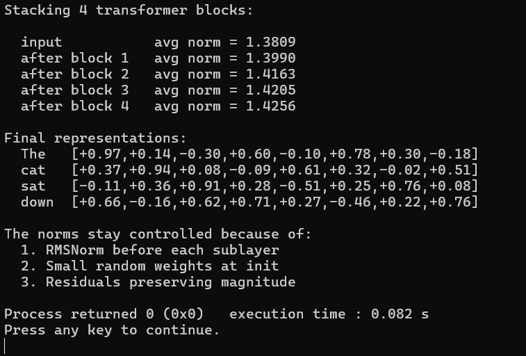
Figure 24-5 stacks four blocks and reports the representation norm at each depth. The average norm across the four positions reads 1.3809 at the input, then 1.3990, 1.4163, 1.4205 and 1.4256 after each of the four blocks in turn. That is a total climb of about three percent across the stack, and the shape of the climb is more informative than its size, because the increments shrink as the depth grows, running 0.018, 0.017, 0.004 and 0.005. The representation is settling rather than compounding, which is the behavior a deep stack needs.
Compare that against the two extremes we produced last chapter and the difference is instructive. There a post-norm stack was pinned at exactly 2.000 at every depth, because the final operation of each layer forced it there, and a pre-norm stack climbed steadily to 43.507 over thirty two layers because nothing constrained it. Neither happens here, and the reason is the near identity behavior from the previous section. Each block adds only a small correction to the running sum, so the sum barely moves over four blocks, and the growth that Chapter 23 measured would only begin to show at eight or sixteen times this depth. Real pre-norm transformers do eventually see that growth, which is why they place one final normalization after the last block rather than relying on the stack to regulate itself.
The program names the three mechanisms holding this together and each is load bearing. RMSNorm gives every sublayer an input at a consistent scale no matter what the residual stream has accumulated by that point, so a sublayer at block sixty sees numbers in the same range as one at block one. Small initial weights keep each sublayer’s contribution to the stream small, which is what makes the near identity start possible. The residual connections carry the representation forward rather than forcing each block to reconstruct it from whatever the previous block emitted. Remove any one of the three and the stack destabilizes in a different way, which exercises 1 and 2 ask you to produce deliberately so that the failure modes are familiar rather than theoretical.
24.7 Parameter Count for Real Models
The two formulas from the block we assembled hold at any scale, so the last program applies them to five real models and sets the computed result against the parameter count each model is actually published with. The gap between those two columns turns out to be the useful part of the exercise.
/* 130_Real_Params.c */
#include <stdio.h>

/* Print a count in a readable unit */
static void human(long long v)
{
    if (v >= 1000000000LL)
        printf("%6.1fB", v / 1e9);
    else if (v >= 1000000LL)
        printf("%6.1fM", v / 1e6);
    else
        printf("%6lldK", v / 1000);
}

int main(void)
{
    struct {
        const char *name;
        int d_model, n_heads, d_ff, n_layers;
        long long published;
    } models[] = {
        { "GPT-2 Small",  768,  12,  3072, 12,
          124000000LL },
        { "GPT-2 Medium", 1024, 16,  4096, 24,
          355000000LL },
        { "GPT-2 Large",  1280, 20,  5120, 36,
          774000000LL },
        { "LLaMA-7B",     4096, 32, 11008, 32,
          6700000000LL },
        { "DeepSeek-V3",  7168, 128, 18432, 61,
          671000000000LL },
    };
    int n = 5, i;

    printf("Transformer block parameters in real "
           "models\n\n");
    printf("  model          d_model  d_ff   L  ");
    printf("per block  all blocks  published\n");
    printf("  -------------  -------  -----  --  ");
    printf("-------  ---------  ---------\n");

    for (i = 0; i < n; i++) {
        int dm = models[i].d_model;
        int df = models[i].d_ff;
        long long attn  = 4LL * dm * dm;
        long long ffn   = 2LL * dm * df;
        long long norms = 2LL * dm;
        long long per   = attn + ffn + norms;
        long long all   = per * models[i].n_layers;

        printf("  %-13s  %7d  %5d  %2d  ",
               models[i].name, dm, df,
               models[i].n_layers);
        human(per);   printf("  ");
        human(all);   printf("  ");
        human(models[i].published);
        printf("\n");
    }

    printf("\n  The last two columns disagree, and "
           "the\n");
    printf("  gap is what the block accounting "
           "leaves\n");
    printf("  out. Token embeddings, the output "
           "head\n");
    printf("  and the final norm all sit outside "
           "the\n");
    printf("  blocks. For GPT-2 Small the embedding\n");
    printf("  table alone is 50257 x 768, about "
           "39M.\n\n");

    printf("  DeepSeek-V3 is the extreme case. Its "
           "FFN\n");
    printf("  is a mixture of experts, so the real\n");
    printf("  count is far above a dense estimate, "
           "and\n");
    printf("  only 37B of the 671B are active per\n");
    printf("  token. Chapter 36 builds that.\n\n");

    printf("  Within a block, attention costs 4*d^2\n");
    printf("  and the FFN costs 2*d*d_ff, so the "
           "FFN\n");
    printf("  dominates whenever d_ff exceeds 2*d.\n");

    return 0;
}
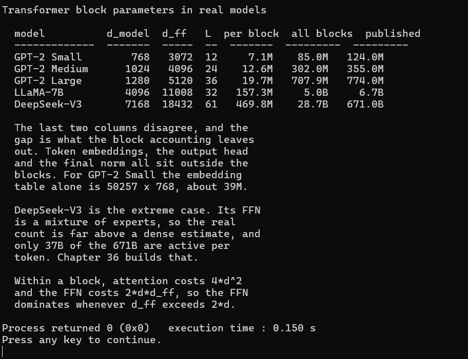
Figure 24-6 sets the computed block parameters against the published model sizes. The rightmost pair of columns disagrees in every row and the disagreement is not an error. GPT-2 Small’s blocks come to 85.0M against a published figure of 124.0M, GPT-2 Large’s come to 707.9M against 774.0M, and LLaMA-7B’s come to 5.0B against 6.7B. In each case the computed number is smaller, and it is smaller by roughly the same kind of margin, which points at something systematic rather than an arithmetic slip.
What the block accounting leaves out is everything that is not a block. A transformer needs an embedding table mapping every token in its vocabulary to a vector, an output head mapping the final vectors back to a score per vocabulary entry, and a final normalization after the last block, and none of those appear in a per block formula. The embedding table is usually the largest of the three by a wide margin, because it scales with vocabulary size rather than with depth. For GPT-2 Small the vocabulary is 50257 entries at 768 dimensions, which comes to 38.6M parameters, and adding that to the 85.0M of blocks gives 123.6M against a published 124.0M. The accounting closes to within half a percent, and the remainder is the positional embedding table and the final norm.
DeepSeek-V3 is the row that does not close, and it fails for a reason worth understanding rather than a reason worth patching. Its blocks compute to 28.7B while the published figure is 671B, a factor of more than twenty rather than the modest gap the other rows show. No embedding table accounts for that. The formula does not apply because DeepSeek-V3 does not have a single feedforward network per block, but a mixture of experts holding many parallel networks of which only a few run for any given token. The 671B counts every expert in the model and the widely quoted 37B counts the ones active per token, so the dense formula used here is measuring something that does not exist in that architecture. Chapter 36 builds the mechanism and the numbers make sense there.
Reading down the per block column shows the other lesson. The cost grows from 7.1M at a model dimension of 768 to 469.8M at 7168, and since both terms in the formula are proportional to d_model squared or to d_model times d_ff, and d_ff itself scales with d_model, doubling the width roughly quadruples the cost of every block in the stack. That quadratic relationship is why model dimensions have grown slowly across generations while layer counts and training set sizes have grown fast, since adding depth costs linearly and adding width does not.
24.8 What You Have Built
The block now standing is the one in current use. Pre-norm placement with RMSNorm, multi-head self-attention with scaled dot-product scores, a widening feedforward network with a smooth activation, and residual connections around both sublayers. Take this block, put an embedding table and a positional encoding in front of a stack of them, put a normalization and an output projection behind, and the result is the architecture of every major language model of the last several years, differing between models mainly in the numbers plugged into d_model, d_ff, the head count and the depth.
It is not the 2017 original, and the differences are worth listing because each was a deliberate change the field made afterward. The largest is placement, since the original normalized after the residual addition rather than before the sublayer, which is the post-norm arrangement we measured last chapter losing seven eighths of its input sensitivity across thirty two layers. Reaching the original block means moving the normalization rather than merely swapping which normalization is used. Beyond that, the original used LayerNorm rather than RMSNorm, so it subtracted the mean and carried a beta parameter alongside gamma, its feedforward network used ReLU where ours uses GELU, and it applied dropout to each sublayer output before the residual addition, which we have omitted entirely because nothing here is being trained. Reverse all four and you have the 2017 encoder block, and every one of those reversals costs training stability at depth, which is why no current model makes them.
What is still missing is only what surrounds the block. There is no embedding table at the front, no output head at the back, and no causal mask inside the attention, which is the single change that turns an encoder block into a decoder block by preventing a position from attending to anything after it. Exercise 4 adds the mask and is worth doing before Chapter 26 rather than after, because the mask is three lines of code and one idea, and having written it yourself makes the decoder-only architecture read as a small modification rather than a new thing. Chapter 25 assembles the encoder-decoder arrangement from the 2017 paper, and Chapter 26 builds the decoder-only stack that every current language model uses.
24.9 Key Takeaways
A transformer block is two sublayers, multi-head attention and a position-wise feedforward network, each wrapped in a normalization applied to its input and a residual addition applied to its output.
Attention is the only place positions interact, so one block gives the sequence exactly one opportunity to move information sideways. Depth compounds that reach, since after two blocks a position knows what its neighbors had already gathered from theirs.
Pre-norm means x = x + Sublayer(RMSNorm(x)), which leaves the residual addition last so that the value carried through the stack is a running sum no normalization ever rescales directly.
The residual derivative is 1 + f’(x) and the leading 1 does not depend on the sublayer at all. Addition is the only common operation whose derivative is exactly one, which is why Chapters 15, 23 and 24 all arrive at it from different directions.
The feedforward network holds more parameters than attention. Attention costs 4 * d_model^2 and the FFN costs 2 * d_model * d_ff, so at the conventional d_ff of four times d_model the FFN costs twice as much as attention does.
An untrained block is close to an identity function, because the residual passes the input through and both sublayers start near zero. We measured every component of every position moving only in the second decimal place.
That near identity start is a feature rather than an accident. Training moves each block a small distance from identity rather than searching for a working function starting from noise, and initialization schemes for deep transformers are designed to preserve it.
Input and output shapes are equal, which is the property that permits stacking and which no other architecture in this book has. We measured the average norm moving from 1.3809 to 1.4256 across four blocks, with the per block increment shrinking rather than compounding.
Per block parameters grow with the square of the model dimension, from 7.1M at 768 to 469.8M at 7168, which is why model widths have grown slowly while depths and dataset sizes have grown quickly.
Block counts do not equal published model sizes, and the gap is the embedding table, the output head and the final norm. GPT-2 Small’s blocks come to 85.0M against 124.0M published, and its 38.6M embedding table closes almost exactly that difference.
DeepSeek-V3 is the exception, with blocks computing to 28.7B against 671B published, because its feedforward network is a mixture of experts of which only 37B are active for any given token.
24.10 Exercises
Remove the residual connections from 128_Block.c and run it. What happens to the output magnitudes? What about with 4 stacked blocks?
Remove the RMSNorm from 128_Block.c and run it. How does the output change? Try stacking 4 blocks without normalization.
Replace GELU with ReLU in the FFN. Does the output change significantly? GELU vs ReLU matters more during training than at inference.
Implement the causal mask, modifying the attention so position i can only attend to positions j <= i. This converts the encoder block into a decoder block (Chapter 26).
Count the total parameters for a 6-layer transformer with d_model=256, n_heads=4, d_ff=1024. How does this compare to the LSTM from Chapter 15 with hidden_size=256?
DeepSeek-V3 uses SwiGLU instead of GELU in its FFN. SwiGLU uses three weight matrices instead of two, so `output = (W1*x * sigmoid(W3*x)) * W2`. Implement this and count the parameters.