Reinforcement Learning
States, actions, rewards, and policies
28.1 What You Will Learn
Every network in this book so far has been trained the same way, whatever else changed around it. Somebody supplied the right answer, the model produced its own answer, and the difference between the two became a gradient that moved the weights. That arrangement works whenever the right answer exists and is cheap to obtain, which covers image labels, translation pairs and the next token in a corpus of text, and it is the reason supervised learning carried the field all the way to Chapter 27 without needing anything else.
It stops working the moment nobody knows the right answer. Consider asking a model to write a helpful reply to a difficult question. There is no single correct reply to compare against, no way to write one down for every possible input, and no procedure that would generate them at the scale training requires. What there is instead is a person who can read two candidate replies and say which of the two is better. That is a score rather than a target, and turning scores into gradients is the entire business of reinforcement learning.
The vocabulary is different enough to be worth building carefully. An agent observes a state, chooses an action, receives a reward, and finds itself in a new state, and the thing being learned is a policy, which is a rule for choosing actions. This chapter builds each of those in C on an environment small enough to verify by hand, then implements REINFORCE, which is the simplest algorithm that turns rewards into gradients. The chapter closes on the tension between using what you already know and finding out what you do not.
None of this is a detour from the transformer material. Chapter 33 aligns a language model to human preferences, and the mapping across is exact rather than analogical. The state is the text generated so far, the action is the choice of next token, the policy is the model itself, and the reward comes from a separate model trained on human comparisons between outputs. Every term in that sentence gets its definition in this chapter, and the algorithm Chapter 33 uses is a refinement of the one we build here rather than a different thing.
28.2 The Setup
Supervised learning needs pairs of an input and its correct output, and the whole apparatus is built around having both halves of every pair. Reinforcement learning throws that away and replaces it with a loop between two parties. The agent is whatever makes decisions, which throughout this book means a neural network. The environment is everything else, meaning the part of the world that responds to what the agent does, and it may be a simulator, a game, a robot’s surroundings or a scoring function. Three quantities pass between them, a state describing the current situation, an action chosen by the agent, and a reward the environment returns to score what just happened.
The loop runs until the episode ends. The agent sees a state, picks an action, and the environment answers with a reward and whatever state the world is in afterward. What makes this harder than supervised learning is the shape of the feedback rather than its quantity. A supervised loss compares an output against a target and therefore points in a direction, telling the optimizer not merely that something was wrong but which way to move. A reward is one number describing the action actually taken, and it says nothing whatsoever about what a better action would have been, so the direction has to be inferred by trying things and comparing outcomes.
The goal is a policy, meaning a rule that maps each state to a choice of action, and specifically the policy that maximizes the total reward collected across a whole episode rather than the reward collected at any single step. That distinction is where the entire difficulty of the field comes from. An action with a poor immediate reward can lead to a state from which far better rewards become available, so a greedy agent that maximizes the next number it sees will walk straight past the good outcomes. Chess makes the point plainly, since sacrificing a piece scores badly on the next move and wins the game several moves later, and any agent that cannot represent that trade cannot play.
28.3 A Simple Environment
The environment here is a line of five positions and nothing else. The agent starts at position 0, can move left or right on each turn, and bumps into a wall if it tries to go left from where it started. Every move costs −1, with one exception, which is that a move landing on position 4 pays +10 instead of costing anything. That exception is the detail to hold onto through the next three sections, because the goal reward replaces the step penalty rather than being added on top of it, and the difference shows up as an off-by-one in the total that the original version of this chapter got wrong in two places.
/* 144_Environment.c */
#include <stdio.h>

#define GRID_SIZE 5
#define GOAL 4

typedef struct {
    int position;
    int done;
}
State;

typedef struct {
    int reward;
    State next_state;
}
StepResult;

/* Actions: 0 = left, 1 = right */
static StepResult env_step(State s, int action)
{
    StepResult r;
    r.next_state = s;
    r.reward = -1;  /* step penalty */

    if (action == 1 && s.position < GRID_SIZE - 1)
        r.next_state.position++;
    else if (action == 0 && s.position > 0)
        r.next_state.position--;

    if (r.next_state.position == GOAL) {
        r.reward = 10;
        r.next_state.done = 1;
    }

    return r;
}

int main(void)
{
    State s = { .position = 0, .done = 0 };
    int total_reward = 0;
    int step;

    printf("Grid world, 5 positions, goal at %d\n",
           GOAL);
    printf("  Actions: 0=left, 1=right\n");
    printf("  Rewards: -1 per step, +10 at goal\n\n");

    /* Hardcoded policy: always go right */
    printf("  step  pos  action  reward  total\n");
    printf("  ----  ---  ------  ------  -----\n");
    for (step = 0; !s.done && step < 10; step++) {
        int action = 1;  /* always right */
        StepResult r = env_step(s, action);
        total_reward += r.reward;
        printf("  %3d    %d    right   %+3d    %+3d\n",
               step, s.position, r.reward,
                   total_reward);
        s = r.next_state;
    }

    /* The move that lands on the goal pays +10
       in place of the -1, so a %d step run costs
       %d penalties and collects 10 */
    printf("\n  Total reward: %d\n", total_reward);
    printf("  Best possible: %d steps, %d at -1, "
           "then +10 = %d\n",
           GOAL, GOAL - 1, -(GOAL - 1) + 10);

    return 0;
}
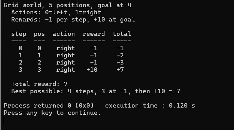
Figure 28-1 walks one optimal run through the grid world. The trace shows four moves and a total of 7. Three of those moves cost −1 each, taking the running total to −3, and the fourth lands on the goal and pays +10, which brings it to +7. The last line reports the best possible outcome using the same breakdown, four steps of which three are penalties, and it agrees with the run.
Being precise about that is worth the trouble because the obvious formula gives a different answer. Four steps at −1 plus a goal reward of 10 comes to 6, and 6 is what you get if the goal move costs a penalty as well as paying out. This environment does not work that way, so the correct figure is 7, and we confirm it independently in a moment by measuring what an optimal policy actually collects over a thousand episodes.
The design of the reward is worth a moment of its own, since it is the part of a reinforcement learning problem that a practitioner actually chooses. The +10 at the goal tells the agent where to go. The −1 per step tells it to get there quickly, and without that penalty every policy that eventually reaches position 4 would score the same 10, including one that wanders for a thousand moves first. Reward design is where most of the difficulty in applied reinforcement learning lives, because an agent optimizes exactly what you wrote down rather than what you meant.
What makes this a learning problem rather than an arithmetic problem is that the agent is not told any of the above. It does not know that position 4 is special, that left is a wasted move, or even that the positions form a line. It knows only which state it is in, which actions exist, and what number came back after it acted.
28.4 Policies, Random and Otherwise
A policy is a mapping from states to action probabilities rather than from states to single actions, and the distinction matters more than it looks. Probabilities allow the same policy to behave differently on two runs, which is what makes exploration possible at all, and a deterministic policy is simply the special case where one probability is 1 and the rest are 0. This program writes down three policies over the environment from 144_Environment.c, runs each of them for a thousand episodes, and averages what they collect.
/* 145_Policy.c */
#include <stdio.h>
#include <stdlib.h>

#define GRID_SIZE 5
#define GOAL 4
#define N_ACTIONS 2

static float randf(void)
{
    return (float)rand() / RAND_MAX;
}

typedef struct {
    int position;
    int done;
}
State;

/* Policy: probability of going right at each
   position */
typedef struct {
    float prob_right[GRID_SIZE];
}
Policy;

static int sample_action(const Policy *p, int pos)
{
    return (randf() < p->prob_right[pos]) ? 1 : 0;
}

static int run_episode(const Policy *p, int verbose)
{
    State s = { .position = 0, .done = 0 };
    int total = 0, step;

    for (step = 0; !s.done && step < 20; step++) {
        int action = sample_action(p, s.position);
        int reward = -1;
        if (action == 1 && s.position < GRID_SIZE - 1)
            s.position++;
        else if (action == 0 && s.position > 0)
            s.position--;
        if (s.position == GOAL) {
            reward = 10;
            s.done = 1;
            }
        total += reward;

        if (verbose)
            printf("    step %d: pos=%d action=%s "
                   "reward=%+d\n",
                   step, s.position,
                   action ? "right" : "left", reward);
    }
    return total;
}

int main(void)
{
    int i, trial;

    /* Random policy */
    Policy random_p;
    for (i = 0; i < GRID_SIZE; i++)
        random_p.prob_right[i] = 0.5f;

    /* Good policy */
    Policy good_p;
    for (i = 0; i < GRID_SIZE; i++)
        /* almost always go right */
        good_p.prob_right[i] = 0.9f;

    /* Optimal policy */
    Policy optimal_p;
    for (i = 0; i < GRID_SIZE; i++)
        /* always go right */
        optimal_p.prob_right[i] = 1.0f;

    printf("Policies averaged over 1000 "
           "episodes\n\n");

    struct { const char *name; Policy
        *p;
        }
        policies[] = {
        { "Random (50/50)", &random_p },
        { "Good, 90% right", &good_p },
        { "Optimal, 100% right", &optimal_p },
    };

    srand(42);
    for (i = 0; i < 3; i++) {
        float avg = 0;
        for (trial = 0; trial < 1000; trial++)
            avg += run_episode(policies[i].p, 0);
        avg /= 1000;
        printf("  %-22s  avg reward = %+.1f\n",
               policies[i].name, avg);
    }

    printf("\n  The optimal policy reaches the goal "
           "in %d steps.\n", GOAL);
    printf("  A random policy wastes steps on left.\n");
    printf("  The job of RL is finding that policy "
           "from experience.\n");

    return 0;
}
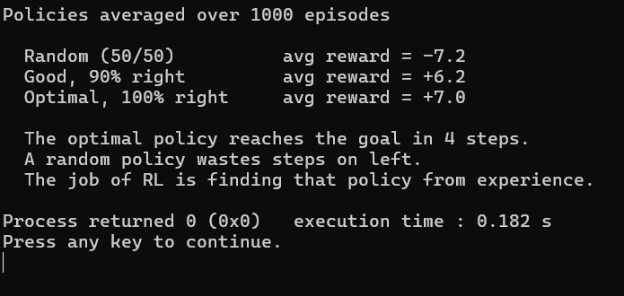
Figure 28-2 averages three policies over a thousand episodes each. The three averages separate cleanly and the spread is larger than the differences between the policies would suggest. A random policy that goes each way with equal probability averages −7.2. A policy that goes right ninety percent of the time averages +6.2. One that always goes right averages +7.0. The last figure is the independent confirmation promised in the previous section, since a policy that cannot make a mistake collects exactly the 7 that the optimal trace produced, which settles the question of whether the total should have been 6 or 7.
Look at the gap between the random policy and the other two, because the sign is the interesting part rather than the size. A random walk on this line does eventually reach position 4, so it always collects the +10 in the end, and it still averages a loss of 7.2. The step penalties overwhelm the goal reward because a random walk takes many more than four steps to travel four positions, which is a standard result about random walks and the reason the penalty was put there.
The ninety percent policy is the one worth studying, because it is what a partially trained agent looks like. One wrong move in ten is enough to cost 0.8 of average reward, and the loss is worse than the arithmetic first suggests, since a leftward move costs a penalty going out and another coming back and leaves the agent no closer than before. Errors in a sequential problem compound in a way that errors in a classification problem do not.
None of these three policies was learned. All three were written down by someone who already knew that right is the correct direction, which is precisely the knowledge a reinforcement learning agent is not given and has to acquire. The rest of the chapter is about reaching that third row from nothing, and the measurement to beat is the +7.0 sitting in it.
28.5 Return and Discounting
The quantity an agent maximizes is the return, meaning the total reward collected from a given point to the end of the episode rather than the reward collected at that step. Most formulations discount it, weighting a reward at the next step by gamma, the one after by gamma squared, and so on.
Gamma sits between 0 and 1 and sets how far ahead the agent cares to look. At 1 it weighs a reward a hundred steps away exactly as heavily as one available immediately, and at 0 it is blind to everything beyond the current step. Values in between produce a soft horizon, where rewards fade in importance the further off they are, and the rate of that fading is the only thing gamma controls.
/* 146_Return.c */
#include <stdio.h>
#include <math.h>

int main(void)
{
    /* A sequence of rewards */
    /* One optimal run of the Step 1 environment,
       three moves at -1 then the goal move at +10 */
    float rewards[] = { -1, -1, -1, 10 };
    int n = (int)(sizeof(rewards) / sizeof(rewards[0]));
    int i, j;

    printf("Discounted return computation:\n\n");
    printf("  Rewards: [");
    for (i = 0; i < n; i++)
        printf("%.0f%s", rewards[i],
               i<n-1?", ":"");
    printf("]\n\n");

    float gammas[] = { 1.0f, 0.99f, 0.9f, 0.5f };
    int n_gamma = 4;

    printf("  gamma   G_0 (return from step 0)\n");
    printf("  ------  -----------------------\n");

    for (j = 0; j < n_gamma; j++) {
        float gamma = gammas[j];
        float G = 0;
        for (i = n - 1; i >= 0; i--)
            G = rewards[i] + gamma * G;
        printf("  %.2f    %+.2f\n", gamma, G);
    }

    printf("\n  gamma=1.0 does not discount at all\n");
    printf("  gamma=0.9 makes the +10 at step 3 "
           "worth 10*0.9^3 = %.2f\n",
           10 * powf(0.9f, 3));
    printf("  gamma=0.5 makes it worth "
           "10*0.5^3 = %.2f\n",
           10 * powf(0.5f, 3));
    printf("\n  Lower gamma = more short-sighted "
           "agent.\n");
    printf("  Higher gamma = plans further ahead.\n");

    return 0;
}
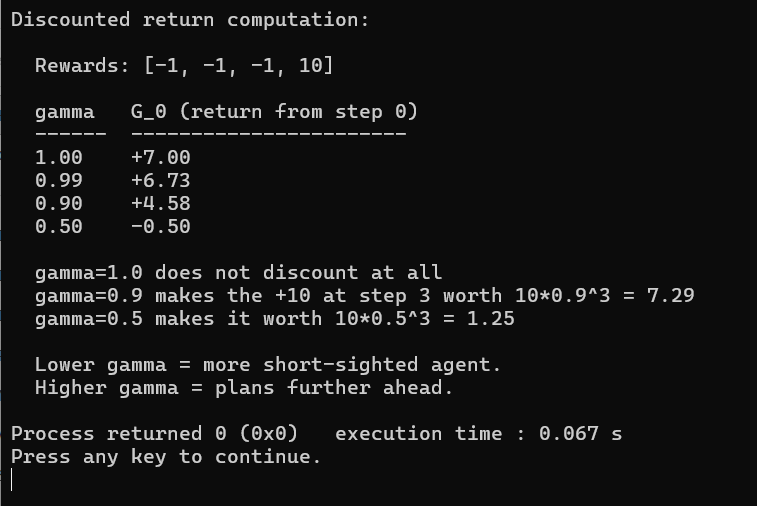
Figure 28-3 discounts the same rewards at four values of gamma. The reward sequence is one optimal run of the grid world, three moves at −1 followed by the goal move at +10, and the table computes the return from step 0 at four values of gamma. At gamma of 1.00 the return is +7.00, which matches what the environment and the policies already gave us, since no discounting means the return is simply the sum. Drop to 0.99 and it falls to +6.73, drop to 0.90 and it falls to +4.58, and at 0.50 it turns negative at −0.50.
The two explanatory lines underneath show exactly where the collapse comes from, and it is an asymmetry rather than a uniform shrinking. The +10 arrives three steps in, so it gets multiplied by gamma cubed, which is 7.29 at a gamma of 0.90 and only 1.25 at a gamma of 0.50. The penalties, meanwhile, arrive at steps 0, 1 and 2 and are barely discounted at all, with the first one not discounted whatsoever. Lowering gamma therefore shrinks the reward hard while leaving the costs almost intact, and at 0.50 the goal has become worth less than the journey to reach it. An agent optimizing that return would rather stand still than walk to the prize.
That is not a flaw in discounting, it is discounting working. A low gamma produces a short-sighted agent by design, and there are problems where that is what you want, particularly where the far future is genuinely unpredictable and planning for it is wasted effort. What the table shows is how sharply the horizon moves, since a change from 0.99 to 0.90 sounds small and cuts the effective planning distance by roughly a factor of ten.
There is a practical reason discounting exists at all beyond modelling preference. An episode that never ends has an infinite undiscounted return, which no algorithm can optimize, and any gamma below 1 makes that sum converge. For episodes that terminate, as this one does, gamma is a modelling choice rather than a mathematical necessity, and gamma of 1 is perfectly legitimate.
28.6 Policy Gradient with REINFORCE
Here is the difficulty this whole chapter has been circling. Backpropagation needs a loss, a loss needs a target, and reinforcement learning has no target by definition, so there is nothing to subtract the output from and no obvious place for a gradient to come from. REINFORCE produces one anyway, using a trick simple enough that it looks like a mistake the first time you meet it.
Run an episode and record every action taken. Compute the return. Then, for each action, nudge the policy to make that action more likely if the return was good and less likely if it was bad, scaling the nudge by the return itself. Good outcomes reinforce whatever produced them and bad outcomes suppress it. No supervisor is required at any point.
/* 147_Reinforce.c */
#include <stdio.h>
#include <stdlib.h>
#include <math.h>

#define GRID_SIZE 5
#define GOAL 4
#define N_ACTIONS 2

static float randf(void)
{
    return (float)rand() / RAND_MAX;
}

/* Policy: logit for "go right" at each position */
float policy_logits[GRID_SIZE];

static float sigmoid(float z)
{
    return 1.0f / (1.0f + expf(-z));
}

static int sample_action(int pos)
{
    float prob_right = sigmoid(policy_logits[pos]);
    return (randf() < prob_right) ? 1 : 0;
}

/* Store an episode */
#define MAX_STEPS 30
static int ep_positions[MAX_STEPS];
static int ep_actions[MAX_STEPS];
static float ep_rewards[MAX_STEPS];
static int ep_len;

static float run_episode(void)
{
    int pos = 0;
    float total = 0;
    ep_len = 0;

    int step;
    for (step = 0; step < MAX_STEPS; step++) {
        int action = sample_action(pos);
        ep_positions[ep_len] = pos;
        ep_actions[ep_len] = action;

        float reward = -1;
        if (action == 1 && pos < GRID_SIZE - 1) pos++;
        else if (action == 0 && pos > 0) pos--;
        if (pos == GOAL) {
            reward = 10;
            }

        ep_rewards[ep_len] = reward;
        total += reward;
        ep_len++;

        if (pos == GOAL) break;
    }
    return total;
}

static void update_policy(float lr)
{
    /* Compute returns (backward) */
    float returns[MAX_STEPS];
    float G = 0;
    int t;

    for (t = ep_len - 1; t >= 0; t--) {
        G = ep_rewards[t] + 0.99f * G;
        returns[t] = G;
    }

    /* Policy gradient: increase prob of good actions */
    for (t = 0; t < ep_len; t++) {
        int pos = ep_positions[t];
        int action = ep_actions[t];
        float prob_right = sigmoid(policy_logits[pos]);

        /* Gradient of log(prob) w.r.t. logit */
        float grad;
        if (action == 1)
            /* d log(sigma(x)) / dx */
            grad = 1.0f - prob_right;
        else
            /* d log(1-sigma(x)) / dx */
            grad = -prob_right;

        /* Scale by return (REINFORCE) */
        policy_logits[pos] += lr * grad * returns[t];
    }
}

int main(void)
{
    int i, ep;
    srand(42);

    /* Initialize policy logits to 0 (50/50 random) */
    for (i = 0; i < GRID_SIZE; i++)
        policy_logits[i] = 0.0f;

    printf("REINFORCE policy gradient training:\n\n");
    printf("  episode   avg_reward   policy, prob "
           "right per pos\n");
    printf("  -------   ----------   -------------"
           "--------------\n");

    for (ep = 0; ep < 500; ep++) {
        float total = 0;
        int batch = 10;
        int b;

        for (b = 0; b < batch; b++) {
            total += run_episode();
            update_policy(0.01f);
        }

        if ((ep + 1) % 100 == 0) {
            printf("  %5d     %+6.1f       [",
                   ep + 1, total / batch);
            for (i = 0; i < GRID_SIZE; i++)
                printf("%.2f%s",
                    sigmoid(policy_logits[i]),
                       i < GRID_SIZE - 1 ? ", " : "");
            printf("]\n");
        }
    }

    printf("\n  The policy converges to a high "
           "prob_right at every\n");
    printf("  position, which is the "
           "optimal policy.\n");
    printf("  No one told the agent to go right. "
           "It found\n");
    printf("  that out from reward signals alone.\n");

    return 0;
}
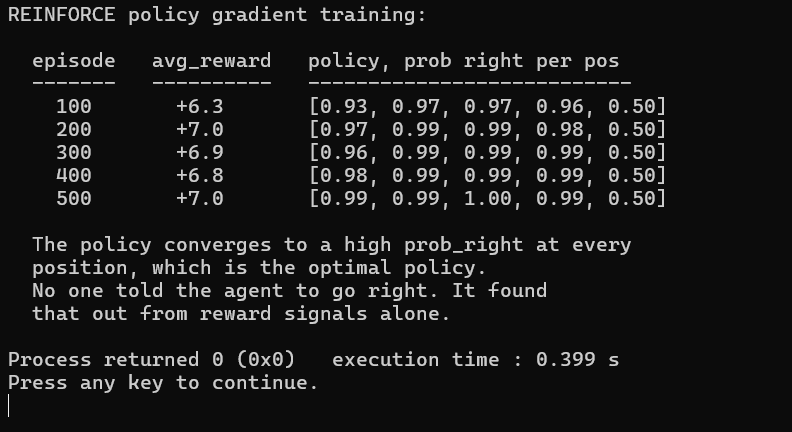
Figure 28-4 has REINFORCE finding the optimal policy from rewards alone. The policy column shows the probability of going right at each of the five positions, and it climbs steadily. After a hundred episodes it reads [0.93, 0.97, 0.97, 0.96, 0.50] and by five hundred it reads [0.99, 0.99, 1.00, 0.99, 0.50], with the average reward settling at +7.0, which is the optimal figure the first three sections established. The agent arrived there from reward signals alone, having never been shown a single correct action.
The fifth entry stays at 0.50 throughout and that is correct rather than a failure to converge. Position 4 is the goal, so the episode ends on arrival and the agent never chooses an action from there, which means no gradient ever reaches that parameter and it keeps its initial value forever. An untouched parameter in a reinforcement learning agent usually means an unreachable state, and noticing them is a useful debugging habit.
Notice how noisy the progress is. Average reward reads +6.3, then +7.0, then +6.9, then +6.8, then +7.0, sliding backward across three consecutive checkpoints even though the policy was strictly improving at every one of them. REINFORCE has famously high variance because it scales every action’s update by the return of the whole episode, so an action that was individually excellent gets punished if the episode went badly for unrelated reasons. Exercise 4 asks you to subtract an average return as a baseline, which is the standard first fix and cuts the variance substantially without biasing the result.
The reason this matters beyond grid worlds is that it is the same machinery Chapter 33 uses. Replace the five positions with the text generated so far, the two actions with a choice over a fifty thousand token vocabulary, and the hand written reward with a model trained to predict human preference, and the algorithm does not change shape. DeepSeek-V3 uses GRPO, which is a variant that computes its baseline by comparing several sampled outputs against each other rather than against a running average, and that is a refinement of the variance problem the paragraph above describes.
28.7 Exploring Against Exploiting
An agent that always takes the action it currently believes is best will never discover that some other action is better, for the straightforward reason that it will never try one. An agent that always tries something new learns a great deal and benefits from none of it. Every reinforcement learning system has to sit somewhere between those two failures, and the position it takes is a decision rather than something the mathematics settles. The simplest workable scheme is epsilon-greedy, which takes the best known action most of the time and a uniformly random action with probability epsilon, and its appeal is that it has exactly one number to tune.
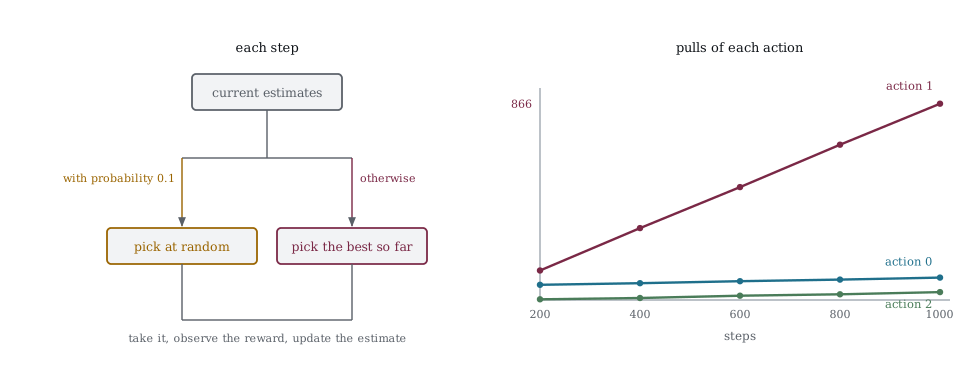
Figure 28-5 shows the rule on the left and its consequence on the right. The decision is a coin flip weighted by epsilon, and everything else follows from it. The right panel plots the pull counts the program prints, which is where the balance becomes concrete.
Action 1 is the best one and takes 866 of the thousand pulls, so the agent is clearly exploiting. The other two still accumulate 99 and 35 pulls, which is the exploration that let it find action 1 in the first place and would let it notice if the rewards changed. Those two lines never flatten, because epsilon is fixed and the agent keeps paying that cost forever.
/* 148_Explore.c */
#include <stdio.h>
#include <stdlib.h>
#include <math.h>

static float randf(void)
{
    return (float)rand() / RAND_MAX;
}

/* Epsilon-greedy. With probability epsilon take a
   random action.
   Otherwise, take the best known action. */

#define N_ACTIONS 3

int main(void)
{
    /* Three slot machines (bandits) with unknown
       payouts */
    float true_rewards[N_ACTIONS] = { 1.0f,
        2.0f, 0.5f };
    float estimated[N_ACTIONS] = { 0, 0, 0 };
    int counts[N_ACTIONS] = { 0, 0, 0 };
    float total = 0;
    int t;

    float epsilon = 0.1f;

    srand(42);

    printf("Epsilon-greedy exploration, "
           "epsilon=%.1f\n\n", epsilon);

    for (t = 0; t < 1000; t++) {
        int action;
        if (randf() < epsilon) {
            /* Explore: random action */
            action = rand() % N_ACTIONS;
        }
        else {
            /* Exploit: best estimated action */
            action = 0;
            int i;
            for (i = 1; i < N_ACTIONS; i++)
                if (estimated[i] > estimated[action])
                    action = i;
        }

        /* Get reward (with noise) */
        float reward = true_rewards[action]
                       + (randf() - 0.5f);
        total += reward;

        /* Update estimate */
        counts[action]++;
        estimated[action] +=
            (reward - estimated[action])
                / counts[action];

        if ((t+1) % 200 == 0) {
            printf("  t=%4d  total=%.0f  "
                   "estimates=[%.2f, %.2f, %.2f]  "
                   "counts=[%d, %d, %d]\n",
                   t+1, total,
                   estimated[0], estimated[1],
                       estimated[2],
                   counts[0], counts[1], counts[2]);
        }
    }

    printf("\n  Action 1 has the highest true "
           "reward at %.1f.\n", true_rewards[1]);
    printf("  The agent found that and exploits it.\n");
    printf("  Epsilon=%.1f means %.0f%% of actions "
           "are exploration.\n",
           epsilon, epsilon * 100);

    return 0;
}
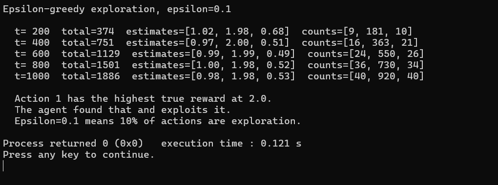
Figure 28-6 balances what the agent knows against what it has not tried. The setup is three actions with fixed true rewards and added noise, and the columns track what the agent believes alongside what it actually does. By a thousand steps the estimates read [0.98, 1.98, 0.53] against true values of 1.0, 2.0 and 0.5, and the counts read [40, 920, 40]. The agent has spent 920 of a thousand steps on action 1, which is the best of the three, while still sampling the other two often enough to keep its estimates of them honest to within a couple of hundredths.
Read the counts against the estimates and the mechanism becomes visible. Action 2 is genuinely the worst of the three and has been tried only 40 times out of a thousand, yet its estimate sits at 0.53 against a true 0.5, which is more than accurate enough to keep rejecting it. The agent does not need a precise measurement of a bad action, only one good enough to rule the action out, and epsilon-greedy ends up allocating its sampling roughly that way without anybody designing it to. Notice also that the two losing actions received 40 draws each, which is close to what pure exploration alone would give them, since epsilon of 0.1 over a thousand steps produces about a hundred random picks split three ways.
The first row shows how quickly the commitment happens. At two hundred steps the counts already read [9, 181, 10], so the agent had put 181 of its first 200 draws into action 1 while having sampled each of the others fewer than a dozen times. Action 2′s estimate at that point was 0.68 against a true 0.5, which is a poor measurement built on ten noisy samples, and the agent was already ignoring it. That is the risk in the scheme, since an action that gets unlucky in its first few trials can be abandoned before it has had a fair hearing. Larger epsilon reduces that risk and costs reward, which exercise 3 asks you to measure across four values.
This problem does not disappear in language models, it changes shape. The temperature sampling from two chapters back is an exploration mechanism, since a temperature of 0 exploits the model’s current beliefs completely and a higher one explores alternatives. During preference training, a policy that has become too confident stops producing the varied outputs a reward model needs to distinguish between, and the standard remedy is a penalty term that keeps the policy from drifting too far from its starting point.
28.8 Key Takeaways
Reinforcement learning replaces the correct answer with a score. An agent observes a state, takes an action, receives a reward, and moves to a new state, and it learns from the numbers rather than from targets.
A reward describes the action that was taken and says nothing about the action that should have been taken. A supervised loss points in a direction, a reward is a single number reporting how things went.
A policy maps states to action probabilities rather than single actions, and a deterministic policy is the case where one probability is 1.
The environment pays +10 in place of the −1 when a move lands on the goal, so an optimal four step run collects 7 rather than the 6 the obvious formula gives. Averaging a thousand episodes confirmed it independently at +7.0.
Reward design is where the difficulty lives. The +10 says where to go and the −1 per step says to hurry, and without the penalty every policy that eventually arrives would score the same.
A random policy averaged −7.2 on this environment despite always reaching the goal eventually, because a random walk takes far more than four steps to cover four positions.
The return is the sum of future rewards, discounted by gamma per step. We measured +7.00 at gamma 1.00 falling to −0.50 at gamma 0.50, because the goal arrives late and is discounted hard while the penalties arrive early and are not.
Discounting also makes the return of a non-terminating episode finite, which is a mathematical necessity rather than a modelling preference.
REINFORCE scales each action’s update by the return of the episode that contained it, making good outcomes more likely and bad ones less. REINFORCE reached [0.99, 0.99, 1.00, 0.99, 0.50] and an average of +7.0 with no supervisor at any point.
The fifth probability stayed at its initial 0.50 because the goal state is never acted from. An untouched parameter usually means an unreachable state.
REINFORCE has high variance because it credits every action in an episode with the whole episode’s outcome. Subtracting a baseline is the standard fix, and GRPO in DeepSeek-V3 builds its baseline by comparing sampled outputs against each other.
Epsilon-greedy took the best known action most of the time and a random one otherwise, spending 920 of 1000 steps on the best action while keeping its estimate of the worst one accurate to 0.53 against a true 0.5 on only 40 samples.
The same terms map onto language model alignment. The state is the text so far, the action is the next token, the policy is the model, and the reward comes from a model of human preference, which is Chapter 33.
28.9 Exercises
Modify 144_Environment.c to add a penalty at position 2 (reward −5). Does the optimal policy change?
Implement a 2D grid world (5x5). The agent can move up, down, left, or right. Goal is at (4,4). Train with REINFORCE.
Try different epsilon values in 148_Explore.c, being 0.01, 0.1, 0.3 and 0.5. Which converges fastest to the optimal action? Which gets the highest total reward?
Implement a baseline subtraction in REINFORCE, where instead of using raw returns, use (return - average_return). This reduces variance and speeds up learning. Compare convergence.
The grid world has a small discrete state space. What happens when the state space is continuous (like a robot’s joint angles)? How would you represent the policy?
Connect this to language modeling, where if the “state” is the sequence generated so far, the “action” is the next token, and the “reward” comes from a human evaluator, you have RLHF. What is the policy in this case?