Q-Learning
Learning action values instead of policies
29.1 What You Will Learn
Chapter 28 learned a policy directly and never learned anything else. The parameters were probabilities of taking each action in each state, REINFORCE nudged them up or down according to how the episode happened to turn out, and at no point did the agent form any opinion about how good a particular state was. Looking at its converged parameters tells you that it goes right from position 1, and tells you nothing about whether position 1 is a good place to be. It knew what to do without knowing why, in the strict sense that nothing anywhere in its weights encoded the fact that position 3 sits closer to the reward than position 0 does.
There is a second approach that inverts the whole arrangement. Rather than learning what to do, learn how much each available option is worth, and then act by picking whichever one is worth the most. The quantity being learned is written Q(s, a), and it estimates the total reward that follows from taking action a in state s and then behaving sensibly for the rest of the episode. A policy falls out of that for free and requires no separate parameters, since knowing the value of every option means the choice is settled by comparison. The agent that results knows why it does what it does, in the sense that its numbers carry a claim about how much each position is worth.
The trick that makes this workable is a recursion, and it is the only real idea in the chapter. The value of an action is the reward it pays immediately, plus the discounted value of the best action available from wherever that action leaves you. That converts a definition which appears to require knowing the answer in advance into one an algorithm can iterate toward from any starting point, because each application of it makes the estimates slightly more consistent with each other than they were. The recursion is called the Bellman equation, it predates neural networks by decades, and everything else in this chapter is machinery around it.
Q-learning is not what aligns language models, and at the end of the chapter we show precisely where the approach runs out of room, which happens long before it reaches a vocabulary of fifty thousand tokens. Building it anyway earns its place twice over. The value based view explains what the policy gradient methods are approximating when they estimate how good an outcome was, and the specific way the method breaks is what motivates both of the escapes the field took afterward. Chapter 30 replaces the table with a network, which fixes one half of the problem, and Chapter 33 abandons values altogether, which is what fixes the other.
29.2 The Q-Value
Q(s, a) answers exactly one question. Standing in state s, taking action a, and then behaving optimally for the remainder of the episode, how much total reward accumulates before it ends? Note that the number is attached to a pair rather than to a state on its own, and the distinction is not cosmetic. The same position in the grid world is worth 10 if you move right from it and considerably less if you move left, so a value indexed only by state could not express the difference between a good square and a good decision. Some formulations do keep a state value alongside, usually written V(s), and it is defined as the Q-value of the best action available there.
Given the full table of Q-values, choosing what to do requires no further thought.
That is simultaneously the appeal of the value based approach and the source of its central difficulty. The definition of Q refers to behaving optimally after the first action, and behaving optimally is precisely what the agent has not yet worked out, so the definition appears to require as input the very thing it exists to produce. Any attempt to compute Q directly from the definition runs immediately into that circularity and stops.
The Bellman equation breaks the circle by making the recursion explicit rather than hiding it.
Read that as a statement about consistency rather than as a formula for computing anything. If a set of Q-values satisfies the equation at every state-action pair simultaneously, those values are the correct ones, and if some pair violates it then the values are wrong and can be improved by moving that particular pair toward what the equation demands. Iterating that correction, pair by pair, in whatever order experience happens to supply them, is the whole of Q-learning. The reason the process converges rather than chasing its own tail is that terminal states anchor it. A state where the episode ends has a value depending on nothing further, so it is correct from the outset, and correctness spreads outward from there one step at a time.
29.3 The Q-Table
For an environment with five states and two actions there are ten Q-values in total, so a table of five rows by two columns holds absolutely everything the agent needs to know about the world. That is the appeal of the tabular approach and, as we will see, the whole of its limitation. This program prints the table as it looks at initialization, then prints the values the Bellman equation says learning ought to arrive at, so the two can be compared against what actually happens in the next section.
/* 149_Qtable.c */
#include <stdio.h>

#define N_STATES 5
#define N_ACTIONS 2  /* 0=left, 1=right */

int main(void)
{
    /* Initialize Q-table to zeros */
    float Q[N_STATES][N_ACTIONS] = {{0}};
    int s, a;

    printf("Initial Q-table (all zeros):\n\n");
    printf("  state   Q(left)   "
           "Q(right)  best action\n");
    printf("  -----   -------   "
           "--------  -----------\n");
    for (s = 0; s < N_STATES; s++) {
        int best = Q[s][1] > Q[s][0] ? 1 : 0;
        printf("  %3d     %+6.2f    %+6.2f    %s\n",
               s, Q[s][0], Q[s][1],
               Q[s][0] == Q[s][1] ? "tie" :
               best ? "right" : "left");
    }

    printf("\n  Every Q-value is zero, so the agent\n");
    printf("  knows nothing at all yet.\n");
    printf("  After learning, Q(s, right) should be\n");
    printf("  higher for states left of the goal.\n");

    /* Work the Bellman equation backward from the
       goal to get the values learning should find */
    printf("\n  What the optimal values are, "
           "gamma=0.9\n\n");

    /* Working backward from goal:
       Q(3, right) = -1 + 0.9*10 = 8.0 (reach goal)
       Q(2, right) = -1 + 0.9*8.0 = 6.2
       Q(1, right) = -1 + 0.9*6.2 = 4.58
       Q(0, right) = -1 + 0.9*4.58 = 3.12 */
    float gamma = 0.9f;
    /* Moving right from state 3 lands on the goal
       and pays +10, ending the episode there, so
       that is where the recursion starts. State 4
       is terminal and no action is taken from it. */
    float ideal[N_STATES];
    ideal[N_STATES-2] = 10.0f;
    for (s = N_STATES - 3; s >= 0; s--)
        ideal[s] = -1 + gamma * ideal[s+1];

    printf("  state   ideal Q(right)\n");
    for (s = 0; s < N_STATES - 1; s++)
        printf("  %3d     %+6.2f\n", s, ideal[s]);
    printf("  %3d     terminal, no action\n",
           N_STATES - 1);

    printf("\n  The values fall with distance from "
           "the goal.\n");
    printf("  Learning has to find these from "
           "experience.\n");

    return 0;
}
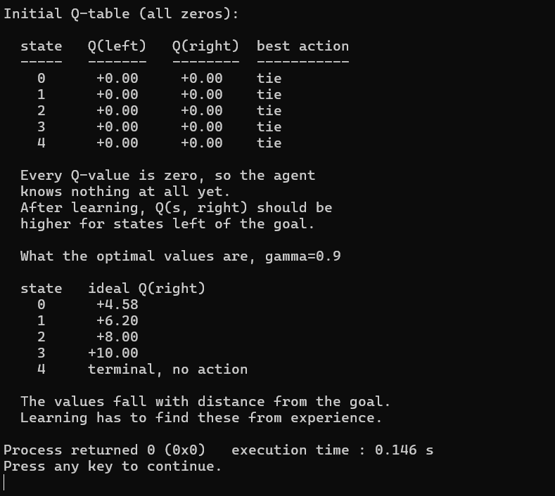
Figure 29-1 has the table before learning beside the values it should reach. The upper table is all zeros and every row reports a tie, which is exactly right for an agent that has seen nothing at all. With no information distinguishing left from right, the argmax has no basis on which to prefer either, and whatever the first action turns out to be is decided by how the tie is broken in code rather than by anything the agent believes. That detail matters more in larger problems than it looks here, because a tie-breaking rule that always picks the lower numbered action introduces a systematic bias into early exploration.
The lower table is the target, worked backward from the goal. Moving right from state 3 lands on position 4 and pays +10, ending the episode, so Q(3, right) is 10 with nothing further to discount. From state 2, moving right costs −1 and delivers the agent to state 3, whose best action is worth 10, so Q(2, right) is −1 plus 0.9 times 10, which is 8.00. The same step gives 6.20 at state 1 and 4.58 at state 0, and the pattern of falling values encodes the distance to the goal without anyone having written down a distance.
State 4 gets no Q-value at all and the table says so. It is the goal, the episode ends on arrival, and an action is never chosen from it, so a value there would be a value for something that never happens. That may seem like pedantry until you notice that including one shifts every other entry by one position, which is a mistake worth being deliberate about avoiding.
Read the falling sequence once more, because it is what the whole method rests on. The agent will never be told that state 3 is close to the goal. It will discover that state 3 is valuable because acting there produces a large reward, then discover that state 2 is valuable because it leads to state 3, and the information propagates backward one state per round of updates. Value based learning is that propagation and nothing else.
29.4 The Update Rule
The Bellman equation describes what correct values look like and says nothing whatsoever about how to find them from a starting point of zeros. The update rule closes that gap in the simplest way available, by taking one small step toward consistency after every single action the agent takes, rather than trying to solve the whole system at once.
The target is what the Bellman equation claims Q(s, a) should be, given the current estimates. The difference between that and the stored value is the error, and alpha decides how much of the error to correct on this step. Small alpha moves slowly and tolerates noise, large alpha moves fast and can oscillate.
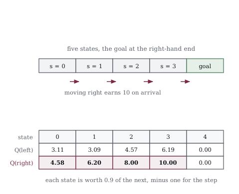
Figure 29-2 shows what those two lines produce after five hundred episodes. Q(s, right) beats Q(s, left) in every state, which is the policy, and the values fall with distance from the goal, which is the discounting.
The right-hand column is worth checking by hand, because the numbers are not arbitrary. Reaching the goal from state 3 pays 10. State 2 is one step further out, so it is worth 0.9 times 10 minus the 1 the step costs, which is 8. State 1 gives 0.9 times 8 minus 1, or 6.2, and state 0 gives 4.58. The table the program prints matches those to the second decimal, so the update rule has recovered the Bellman values without ever being told what they were.
/* 150_Qlearning.c */
#include <stdio.h>
#include <stdlib.h>

#define N_STATES 5
#define N_ACTIONS 2
#define GOAL 4

static float randf(void)
{
    return (float)rand() / RAND_MAX;
}

static float max_q(float Q[N_STATES][N_ACTIONS], int s)
{
    return Q[s][0] > Q[s][1] ? Q[s][0] : Q[s][1];
}

int main(void)
{
    float Q[N_STATES][N_ACTIONS] = {{0}};
    float alpha = 0.1f;   /* learning rate */
    float gamma = 0.9f;   /* discount factor */
    float epsilon = 0.2f; /* exploration rate */
    int episode, step, s, a;

    srand(42);

    printf("Q-learning on grid world:\n\n");

    for (episode = 0; episode < 500; episode++) {
        s = 0;  /* start at position 0 */

        for (step = 0; step < 20; step++) {
            /* Epsilon-greedy action selection */
            if (randf() < epsilon)
                a = rand() % N_ACTIONS;
            else
                a = Q[s][1] > Q[s][0] ? 1 : 0;

            /* Take action */
            int s_next = s;
            if (a == 1 && s < N_STATES - 1)
                s_next = s + 1;
            else if (a == 0 && s > 0) s_next = s - 1;

            float reward = -1;
            int done = 0;
            if (s_next == GOAL) {
                reward = 10;
                done = 1;
                }

            /* Q-learning update */
            float target = reward;
            if (!done)
                target += gamma * max_q(Q, s_next);

            Q[s][a] += alpha * (target - Q[s][a]);

            s = s_next;
            if (done) break;
        }

        if ((episode + 1) % 100 == 0) {
            printf("  Episode %3d:\n", episode + 1);
            printf("    state  Q(left)  Q(right)  "
                   "best\n");
            for (s = 0; s < N_STATES; s++) {
                int best = Q[s][1] > Q[s][0] ? 1 : 0;
                printf("    %3d    %+6.2f   %+6.2f    "
                       "%s\n",
                       s, Q[s][0], Q[s][1],
                       best ? "right" : "left");
            }
            printf("\n");
        }
    }

    printf("  The Q-values reach the optimal ones.\n");
    printf("  Q(s, right) > Q(s, left) for all "
           "states.\n");
    printf("  Q(s, right) falls with distance from "
           "the goal.\n");

    return 0;
}
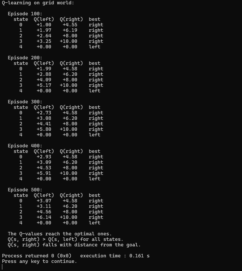
Figure 29-3 follows the Q-values converging over five hundred episodes. By episode 500 the table reads 4.58, 6.20, 8.00 and 10.00 in the right column for states 0 through 3, which matches the Bellman calculation we did by hand to the digit. Right beats left at every state. The agent was never told which direction was correct and never saw a single labelled example.
Watch the order in which the two columns settle. At episode 100 the right column already reads 4.55, 6.19, 8.00 and 10.00, which is essentially converged, while the left column is still scattered at 1.00, 1.97, 2.64 and 3.25. By episode 500 the left column has climbed to 3.07, 3.11, 4.56 and 6.14 and has not finished moving. That asymmetry is the epsilon-greedy policy showing through, since the agent takes the right action most of the time and therefore gathers far more data about it, and the left column improves only on the ten percent of steps that explore.
The left column repays a look rather than a skip, because it is not junk. Q(3, left) reaches 6.14 and is still rising toward 6.2, which is the correct value for moving away from the goal at state 3, since that pays −1 and lands the agent in state 2 whose best action is worth 8, giving −1 plus 0.9 times 8. The agent has learned an accurate value for an action it will never choose, which is the signature of an off-policy method.
That word is the important one in this section. Q-learning updates toward max over the next state’s actions, meaning the best action available there, regardless of what the agent actually did next. A random exploratory move still produces a valid update about the greedy policy. REINFORCE cannot do that, since it learns from the actions it took and nothing else, so every exploratory step in Chapter 28 was a step spent learning about a policy the agent was trying to move away from.
29.5 Against REINFORCE
Both methods solve the same problem and arrive at the same policy, so the interesting comparison is not whether they work but how quickly. Running them side by side on the same environment, with the same reward structure and the same exploration rate, answers that directly and also exposes what the off-policy property is actually worth in practice.
/* 151_Compare.c */
#include <stdio.h>
#include <stdlib.h>
#include <math.h>

#define N_STATES 5
#define GOAL 4
#define N_ACTIONS 2
#define MAX_STEPS 20

static float randf(void)
{
    return (float)rand() / RAND_MAX;
}
static float sigmoid(float z)
{
    return 1.0f / (1.0f + expf(-z));
}

/* --- Q-learning --- */
static float eval_qlearning(int n_episodes)
{
    float Q[N_STATES][N_ACTIONS] = {{0}};
    float alpha = 0.1f, gamma = 0.9f, epsilon = 0.1f;
    float total = 0;
    int ep, step;

    for (ep = 0; ep < n_episodes; ep++) {
        int s = 0;
        float ep_reward = 0;
        for (step = 0; step < MAX_STEPS; step++) {
            int greedy = Q[s][1] > Q[s][0] ? 1 : 0;
            int a = (randf() < epsilon)
                    ? rand() % 2 : greedy;
            int sn = s;
            if (a==1 && s<N_STATES-1) sn = s+1;
            else if (a==0 && s>0) sn = s-1;
            float r = -1;
            int done = 0;
            if (sn==GOAL) {
                r = 10;
                done = 1;
                }
            float best = Q[sn][0] > Q[sn][1]
                         ? Q[sn][0] : Q[sn][1];
            float target = done ? r : r + gamma * best;
            Q[s][a] += alpha * (target - Q[s][a]);
            ep_reward += r;
            s = sn;
            if (done) break;
        }
        if (ep >= n_episodes - 100) total += ep_reward;
    }
    return total / 100;
}

/* --- REINFORCE --- */
static float eval_reinforce(int n_episodes)
{
    float logits[N_STATES] = {0};
    float total = 0;
    int ep, step;

    for (ep = 0; ep < n_episodes; ep++) {
        int positions[MAX_STEPS], actions[MAX_STEPS];
        float rewards[MAX_STEPS];
        int len = 0, s = 0;
        float ep_reward = 0;

        for (step = 0; step < MAX_STEPS; step++) {
            int a = (randf() < sigmoid(logits[s]))
                ? 1
                : 0;
            positions[len] = s;
            actions[len] = a;
            if (a==1 && s<N_STATES-1) s++;
            else if (a==0 && s>0) s--;
            float r = -1;
            if (s==GOAL) r = 10;
            rewards[len] = r;
            ep_reward += r;
            len++;
            if (s==GOAL) break;
        }

        float G = 0;
        for (step = len-1; step >= 0; step--) {
            G = rewards[step] + 0.99f * G;
            float pr = sigmoid(logits[positions[step]]);
            float grad = actions[step]==1
                ? (1-pr)
                : (-pr);
            logits[positions[step]] += 0.01f * grad * G;
        }

        if (ep >= n_episodes - 100) total += ep_reward;
    }
    return total / 100;
}

int main(void)
{
    int trials[] = { 100, 200, 500, 1000 };
    int n = 4, i;

    printf("Q-Learning against REINFORCE, average "
           "over the last 100\n\n");
    printf("  Episodes   Q-Learning   REINFORCE\n");
    printf("  --------   ----------   ---------\n");

    for (i = 0; i < n; i++) {
        srand(42);
        float ql = eval_qlearning(trials[i]);
        srand(42);
        float rf = eval_reinforce(trials[i]);
        printf("  %5d      %+6.1f       %+6.1f\n",
               trials[i], ql, rf);
    }

    printf("\n  Both converge to the "
           "optimal policy.\n");
    printf("  Q-learning learns values, off-policy.\n");
    printf("  REINFORCE learns a policy, on-policy.\n");
    printf("  For LLMs the policy gradient methods\n");
    printf("  win, because the vocabulary is far\n");
    printf("  too large for a Q-table.\n");

    return 0;
}
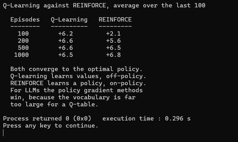
Figure 29-4 runs Q-learning against REINFORCE on the same environment. Q-learning is ahead early and the ordering does not survive. At a hundred episodes Q-learning averages +6.2 while REINFORCE manages only +2.1, which is a third as much. By two hundred the figures are +6.6 and +5.6, and by five hundred they are +6.6 and +6.5. At a thousand episodes REINFORCE has passed it, reading +6.8 against Q-learning’s +6.5.
Do not read much into that final crossing, since both methods are bouncing around the same value and a gap between +6.5 and +6.8 on a hundred episode average is noise rather than a result. What the table does establish is the shape of the early curve, and the shape is the real distinction. Q-learning reaches a good policy in a fraction of the episodes REINFORCE needs, and on any problem where an episode is expensive to run, that is the property deciding which method you can afford.
The early gap is the off-policy property paying off. Q-learning extracts a usable update from every step including the exploratory ones, while REINFORCE waits until an episode finishes and then credits every action in it with the outcome of the whole, which is both slower and noisier. We saw that noise directly last chapter, with average reward moving backward across three consecutive checkpoints while the policy was improving throughout.
Both settle at +6.6 rather than the +7.0 that Chapter 28 established as optimal, and the shortfall is not a failure to converge. Exploration is still running, so roughly a tenth of the actions are random, and a random action costs the agent a step in the wrong direction plus another to undo it. The policy is optimal and the measured behavior is not, because the measurement includes the exploration. Turning epsilon to zero after training would recover the full +7.0 and would also stop the agent learning anything further, which is the trade we described last chapter.
The last lines of the output point where the chapter is going. For a language model the action space is the vocabulary, and Q-learning requires a value per action, so the method needs a number for every one of fifty thousand tokens at every position. Policy gradient methods produce a distribution over that vocabulary directly, which the model already does, and that is the difference that decided which approach the field uses.
29.6 Why Q-Tables Do Not Scale
A table needs one entry per state-action pair, so the memory it requires is the size of the state space multiplied by the size of the action space. That product stays manageable for a very short while.
| Problem | States | Actions | Table entries |
|---|---|---|---|
| Grid world, 5 by 1 | 5 | 2 | 10 |
| Grid world, 10 by 10 | 100 | 4 | 400 |
| Chess | about 10^47 | about 35 | about 10^48 |
| Go | about 10^170 | about 250 | about 10^172 |
| Language model | unbounded | 50,000 | impossible |
The two grid worlds are fine and everything below them is hopeless, with no gradual degradation in between. Chess needs more table entries than there are atoms in the observable universe, a figure usually put at around 10^80, and Go exceeds even that by roughly ninety orders of magnitude. Numbers at that scale are not engineering problems that a larger machine eventually solves, since no arrangement of matter holds the table, and the usual instinct to reach for more memory does not apply.
The language model row is worse than the numbers suggest, because the state is the entire text generated so far, which is not merely large but unbounded, since there is no longest possible prompt. A table indexed by state cannot exist when new states keep being invented, and no amount of compression helps with a set that has no fixed size.
Two escapes exist and the chapter takes one of them next. Replacing the table with a function that computes Q-values on demand removes the storage problem entirely, since a network with a few million weights can produce a value for any state it is shown, including states it has never seen. That is the Deep Q-Network of Chapter 30, and it works well when the action count is small, which for Atari games means a joystick with a handful of positions.
The second escape is to give up on values. A language model already produces a probability distribution over the vocabulary at every position, which is precisely a policy, so training it with policy gradients means adjusting something the model computes anyway rather than bolting on a value head with fifty thousand outputs. That is why Chapter 33 uses REINFORCE and its descendants rather than anything in this chapter, and why the value based path, having been the dominant approach in reinforcement learning for decades, is not the one that aligned the models people actually use.
29.7 Key Takeaways
Q(s, a) is the total reward that follows from taking action a in state s and then behaving optimally. Given the full table, the policy is just the argmax at each state.
The Bellman equation defines Q recursively as the immediate reward plus the discounted best value of the next state. It is a consistency condition rather than a computation, and terminal states anchor it because their values depend on nothing further.
The update rule moves Q toward that target by a fraction alpha of the error, so alpha trades speed against stability.
We worked the values out by hand as 4.58, 6.20, 8.00 and 10.00 for states 0 through 3, and then learned exactly those figures from experience alone.
The goal state has no Q-value because no action is ever taken from it. Inventing one shifts every other entry by a state, which is the kind of off-by-one that produces a plausible looking table full of wrong numbers.
Values propagate backward from the goal, one state per round of updates. The agent discovers that state 3 is valuable because acting there pays, then that state 2 is valuable because it leads to state 3.
Q-learning is off-policy, updating toward the best action available in the next state regardless of what the agent actually did. It reached 6.14 and was still climbing toward the correct 6.2 for a leftward move it would never choose.
REINFORCE is on-policy and learns only from what it actually did, which is why we measured it at +2.1 after a hundred episodes against Q-learning’s +6.2, with the gap closed by five hundred.
Both hover near +6.6 rather than reaching the optimal +7.0 because exploration keeps running throughout. The policy is optimal and the measurement is not, since roughly a tenth of the actions being averaged are deliberately random.
A Q-table needs states times actions entries, which reaches about 10^48 for chess and about 10^172 for Go, against roughly 10^80 atoms in the observable universe.
A language model’s state is unbounded, so no table indexed by state can exist at any size.
Chapter 30 replaces the table with a network, which fixes storage but not a fifty thousand action space. Chapter 33 abandons values entirely and trains the distribution the model already produces.
29.8 Exercises
Run 150_Qlearning.c with gamma = 0.5 instead of 0.9. How do the converged Q-values change? Does the optimal policy change?
Implement SARSA, an on-policy alternative to Q-learning. Instead of using max Q(s’, a’), use Q(s’, a’) where a’ is the action actually taken. Compare convergence.
Add a second goal at position 0 with reward +5. The optimal policy should go left from position 0-1 and right from position 2-4. Does Q-learning discover this?
Implement Q-learning on a 4x4 grid with walls. The agent can move up, down, left, right. Verify that the learned Q-values encode the shortest path around walls.
What happens if alpha is too large (e.g., 1.0)? What about too small (e.g., 0.001)? Try both and compare convergence speed and stability.
Prove that Q-learning converges to the optimal Q-values under certain conditions. What are those conditions? (As a hint, every state-action pair must be visited infinitely often.)