Deep Q-Networks
Replacing the Q-table with a neural network
30.1 What You Will Learn
The last chapter ended by putting a hard number on why the tabular approach stops working. Chess needs roughly 10^48 table entries and Go needs about 10^172, set against perhaps 10^80 atoms in the observable universe, so the failure is not the kind that a larger machine eventually fixes. A table needs one slot per state-action pair, and for any problem worth solving the pairs outnumber anything that could be stored under any physical arrangement of matter. The approach does not scale badly, it stops entirely. The escape is to stop storing the values and start computing them on demand. A network taking a state as input and producing one Q-value per action needs parameters in proportion to its own architecture rather than to the size of the state space, so a few thousand weights can answer a question about a state nobody has ever visited, by interpolating between states that resemble it.
That substitution is the whole idea behind a Deep Q-Network, and stated on its own it would make for a very short chapter.
What makes it a chapter is that the substitution does not work naively, and the two ways it fails are both consequences of a single difference. A table stores independent entries, so writing one changes exactly one value, while a network shares its parameters across every state it will ever be asked about, so writing anything changes everything. Correlated training data becomes dangerous where it was previously harmless, and the Bellman target starts moving under the very updates that chase it. The first is fixed by storing past experience and drawing from it at random, the second by keeping a second copy of the network deliberately out of date, and we build both in this chapter.
DQN is the method that made reinforcement learning work on Atari games from raw pixels, and it is not the method that aligns language models. At the end of this chapter we get to where it runs out, which is a different place from where the table ran out, and that second wall is what sends us back, three chapters from now, to the policy gradients we built in Chapter 28.
30.2 The Idea
The change is a substitution and nothing more. Where in the last chapter we wrote Q[state][action] and read a stored number, a DQN writes network(state) and reads a vector with one entry per action. Everything downstream is untouched, since the Bellman target is computed the same way and the greedy policy is still an argmax over whatever the values turn out to be.
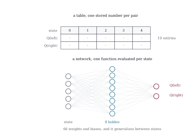
Figure 30-1 puts the two side by side at the sizes this chapter uses. The table is five states by two actions and holds ten numbers, each one independent of the rest. The network takes the state in and returns both Q-values at once from sixty six weights and biases.
For a problem this small the network is the worse deal, since sixty six parameters is more than ten and it has to be trained rather than assigned. The trade only pays when the table stops fitting, and we work out where that happens at the end of the chapter. What the network buys in exchange is on the last line, where touching one weight moves the answer for every state at once, which is the generalization a table can never have.
The second line is what a table never needed. A table entry can be assigned directly, since nothing else depends on it, but a network has no slot to assign, so the correction has to become a loss and reach the weights through backpropagation. That single difference is where the trouble comes from, because gradient descent on shared parameters behaves nothing like writing to an array.
The first problem is correlation. Consecutive states within an episode are nearly identical, so training on them in order feeds the network a long run of almost the same example, and a network fitted to a narrow slice of its input space quietly forgets everything else. A table cannot suffer this, since updating the entry for state 3 leaves the entry for state 0 exactly as it was. Experience replay is the fix, and we build it in the next section.
The second problem is that the target moves. The right hand side of the Bellman equation is computed from the same network being updated, so every gradient step changes both the estimate and the thing it is being pulled toward. A table has this in principle and survives it in practice, because one entry changes at a time. A network changes every value at once, and chasing a target that runs away as you approach is how a DQN diverges. A second frozen copy of the network solves it, and we put that together once the replay buffer is done.
30.3 The Q-Network
The network is a small multilayer perceptron of exactly the kind we built back in Chapter 2, with one hidden layer and nothing unusual anywhere in it. The state arrives as a one-hot vector, five inputs of which exactly one is set to 1, and two outputs come back carrying the estimated value of going left and the estimated value of going right. Nothing about the architecture is specific to reinforcement learning, and the only thing making this a Q-network rather than a classifier is what its outputs are interpreted to mean and what loss is used to train them.
/* 152_Qnetwork.c */
#include <stdio.h>
#include <stdlib.h>
#include <math.h>

static float randf(void)
{
    return (float)rand() / RAND_MAX;
}

#define N_STATES 5
#define N_ACTIONS 2
#define N_HID 8

typedef struct {
    float W1[N_HID][N_STATES];  /* input -> hidden */
    float b1[N_HID];
    float W2[N_ACTIONS][N_HID];
    /* hidden -> Q-values */
    float b2[N_ACTIONS];
}
QNet;

static void qnet_init(QNet *q)
{
    int i, j;
    for (i = 0; i < N_HID; i++) {
        q->b1[i] = 0;
        for (j = 0; j < N_STATES; j++)
            q->W1[i][j] = (randf()*2-1) * 0.3f;
    }
    for (i = 0; i < N_ACTIONS; i++) {
        q->b2[i] = 0;
        for (j = 0; j < N_HID; j++)
            q->W2[i][j] = (randf()*2-1) * 0.3f;
    }
}

static float relu(float x)
{
    return x > 0 ? x : 0;
}

static void qnet_forward(const QNet *q, int state,
                         float qvals[N_ACTIONS])
{
    float h[N_HID];
    int i, j;

    /* One-hot input */
    for (i = 0; i < N_HID; i++) {
        /* one-hot input, so only the column for
           this state contributes anything */
        h[i] = q->b1[i] + q->W1[i][state];
        h[i] = relu(h[i]);
    }
    for (i = 0; i < N_ACTIONS; i++) {
        qvals[i] = q->b2[i];
        for (j = 0; j < N_HID; j++)
            qvals[i] += q->W2[i][j] * h[j];
    }
}

int main(void)
{
    QNet net;
    srand(42);
    qnet_init(&net);

    printf("Q-Network outputs (untrained):\n\n");
    printf("  state   Q(left)   Q(right)  best\n");
    printf("  -----   -------   --------  ----\n");

    int s;
    for (s = 0; s < N_STATES; s++) {
        float qvals[N_ACTIONS];
        qnet_forward(&net, s, qvals);
        printf("  %3d     %+6.3f    %+6.3f    %s\n",
               s, qvals[0], qvals[1],
               qvals[1] > qvals[0] ? "right" : "left");
    }

    printf("\n  Random weights produce random "
           "Q-values.\n");
    printf("  After training these should match the\n");
    printf("  optimal Q-values from Chapter 29.\n");

    int params = N_HID * N_STATES + N_HID
                 + N_ACTIONS * N_HID + N_ACTIONS;
    printf("\n  Parameters: %d (vs %d Q-table "
           "entries)\n",
           params, N_STATES * N_ACTIONS);

    return 0;
}
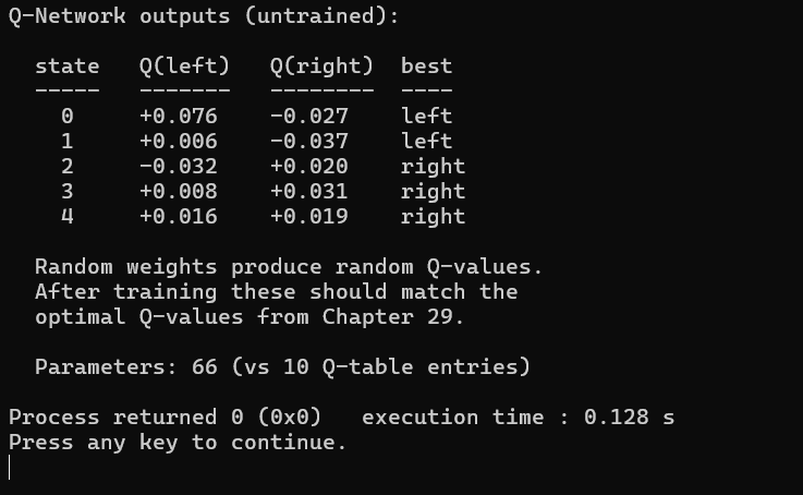
Figure 30-2 has the untrained network beside what it costs against a table. The values are random because the weights are, running between −0.037 and +0.076, and the best action column is therefore meaningless in every row. Two states prefer left and three prefer right on no evidence whatsoever, and reading anything into that split would be reading the random number generator. This is the same starting condition as the all zero table we started from last chapter, with small noise standing in for the zeros, and the noise is preferable because identical outputs give gradient descent nothing to work with.
The parameter count is the line to read twice. Sixty six weights against ten table entries, so on this problem the network is more than six times the size of the thing it replaces, slower to evaluate since every query is two matrix multiplies rather than an array index, and considerably harder to train since it needs a learning rate and can diverge. On a five state grid world the table wins on every measure anybody would care about, and the chapter’s own example is one where its subject matter is plainly the wrong tool.
That inversion is the point rather than an embarrassment. The table costs states times actions and the network costs a figure fixed by its own architecture, so the two curves cross somewhere and everything past the crossing belongs to the network. Add five states to the grid and the table grows by ten entries while the network grows by the width of one hidden layer, which is eight. Take the state space to a million and the table needs two million entries while the network needs the same sixty six, provided the input encoding can address a million states, which one-hot cannot and a sensible feature vector can.
The one-hot encoding is worth noticing for what it gives up. Feeding state 3 as [0,0,0,1,0] means the network sees no relationship between state 3 and state 2, so it learns each state independently and generalizes to nothing. That is a table implemented in floating point, which is exactly the wrong trade, and exercise 4 asks you to replace it with a single scaled number so the network can notice that nearby states are similar.
30.4 Experience Replay
The fix for correlated samples is to stop training in the order things happened. Every transition the agent experiences is written into a circular buffer, and each training step draws a random batch out of that buffer rather than using whatever occurred most recently. A transition is four fields and a flag, being the state the agent was in, the action it took, the reward it received, the state that resulted, and whether the episode ended right there. Those five items are everything the Bellman update needs, which is why a transition can be stored once and reused indefinitely without any record of the episode it belonged to.
/* 153_Replay.c */
#include <stdio.h>
#include <stdlib.h>

#define BUFFER_SIZE 100
#define BATCH_SIZE 8

typedef struct {
    int state;
    int action;
    float reward;
    int next_state;
    int done;
}
Transition;

typedef struct {
    Transition data[BUFFER_SIZE];
    int count;
    int write_pos;
}
ReplayBuffer;

static void rb_init(ReplayBuffer *rb)
{
    rb->count = 0;
    rb->write_pos = 0;
}

static void rb_add(ReplayBuffer *rb, Transition t)
{
    rb->data[rb->write_pos] = t;
    rb->write_pos = (rb->write_pos + 1) % BUFFER_SIZE;
    if (rb->count < BUFFER_SIZE) rb->count++;
}

static void rb_sample(const ReplayBuffer *rb,
                      Transition *batch, int n)
{
    int i;
    for (i = 0; i < n; i++)
        batch[i] = rb->data[rand() % rb->count];
}

/* The Chapter 28 environment, so the buffer
   holds transitions that could really happen */
#define N_STATES 5
#define GOAL 4

static int env_step(int s, int a, float *r,
                    int *done)
{
    int sn = (a == 1) ? s + 1 : s - 1;
    if (sn < 0) sn = 0;      /* wall on the left */
    if (sn > GOAL) sn = GOAL;
    *done = (sn == GOAL);
    *r = *done ? 10.0f : -1.0f;
    return sn;
}

int main(void)
{
    ReplayBuffer rb;
    rb_init(&rb);

    srand(42);

    /* Run episodes with a random policy and store
       every transition the environment produced */
    int i, ep, s = 0;
    for (ep = 0; ep < 6; ep++) {
        int step;
        s = 0;
        for (step = 0; step < 10; step++) {
            /* Lean right so some episodes reach
               the goal and land a done in the buffer */
            int a = (rand() % 10 < 7) ? 1 : 0;
            float r;
            int done;
            int sn = env_step(s, a, &r, &done);
            Transition t;
            t.state = s;
            t.action = a;
            t.reward = r;
            t.next_state = sn;
            t.done = done;
            rb_add(&rb, t);
            s = sn;
            if (done) break;
        }
    }

    printf("Replay buffer: %d transitions stored\n\n",
           rb.count);

    Transition batch[BATCH_SIZE];
    rb_sample(&rb, batch, BATCH_SIZE);

    printf("Random batch of %d transitions\n\n",
           BATCH_SIZE);
    printf("  state  action  reward  next  done\n");
    printf("  -----  ------  ------  ----  ----\n");
    for (i = 0; i < BATCH_SIZE; i++)
        printf("  %3d    %-6s  %+5.0f    %3d   %d\n",
               batch[i].state,
               batch[i].action ? "right" : "left",
               batch[i].reward, batch[i].next_state,
               batch[i].done);

    /* Report what the whole buffer holds, so the
       point does not depend on which rows were drawn */
    int terminal = 0;
    float best = -1e9f;
    for (i = 0; i < rb.count; i++) {
        if (rb.data[i].done) terminal++;
        if (rb.data[i].reward > best)
            best = rb.data[i].reward;
    }
    printf("\n  Buffer holds %d "
           "transitions, of which\n",
           rb.count);
    printf("  %d reached the goal. "
           "Best reward stored\n",
           terminal);
    printf("  is %+.0f. Any batch may "
           "or may not draw\n",
           best);
    printf("  one of those %d, and over many batches\n",
           terminal);
    printf("  each of them is reused many times.\n");

    printf("\n  Every row obeys the environment. "
           "Moving\n");
    printf("  right adds one, moving left subtracts\n");
    printf("  one and stops at the "
           "wall, and done is\n");
    printf("  set only when next is the goal.\n\n");

    printf("  The rows arrive in "
           "shuffled order, so a\n");
    printf("  batch carries no trace "
           "of the episodes\n");
    printf("  it came from. That is "
           "the whole point,\n");
    printf("  since consecutive steps "
           "are correlated\n");
    printf("  and a network trained "
           "on them wobbles.\n");

    return 0;
}
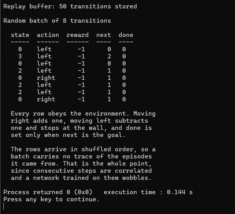
Figure 30-3 shows the buffer holding transitions the environment really produced. It holds several dozen of them gathered over six episodes, and the sampled batch is eight of them in whatever order the draw produced. Check any row against the environment and it holds. Moving right from state 0 gives next state 1 at a cost of −1. Moving left from state 3 gives 2. Moving left from state 0 gives 0 again, because the wall stops the move and the agent still pays the penalty for having tried. Nothing in the table could have come from anywhere but the environment, which was not true of the version this listing replaced.
The summary underneath the table is there because the batch itself may not show the interesting case. It reports how many of the stored transitions actually reached the goal, and that handful carries the only positive reward the environment ever pays. Reaching the goal is uncommon under a near random policy, so an agent training only on recent experience would encounter it, learn from it once, and not see it again for a long stretch. Storing it means the same successful transition can be drawn into twenty separate batches and contribute to twenty updates, which is why replay improves sample efficiency as much as it improves stability.
A batch will often contain the same transition twice, and that is sampling with replacement working as intended rather than a bug. Drawing eight independent samples from a few dozen entries produces at least one duplicate more often than not, which follows from the same argument that makes collisions common in small hash tables. Sampling without replacement avoids it, complicates the code, and buys nothing measurable at this scale, so production implementations generally do not bother either.
Notice what the shuffling destroys. Read the batch top to bottom and you cannot find an episode in it, or a trajectory, or any way to tell which rows came from the same run. A network sees eight unrelated examples spanning the whole state space, which is precisely the independent and identically distributed data that supervised training assumes and that a reinforcement learning agent never naturally produces.
30.5 The Complete DQN
Everything assembles now into one program with four moving parts. A policy network, which is the one being trained and the one that chooses actions, a frozen target network supplying the right hand side of the Bellman equation, a replay buffer feeding random batches rather than recent experience, and an epsilon starting at 0.3 and decaying toward zero as training proceeds, so the agent explores broadly early and commits later.
The target network is the piece that has not appeared yet. It is a copy of the policy network taken every twenty episodes and left untouched in between, and its only job is computing the max over the next state’s values inside the target. Because it does not move between copies, the thing the policy network is being pulled toward stays still long enough to be reached.
/* 154_Dqn.c */
#include <stdio.h>
#include <stdlib.h>
#include <math.h>
#include <string.h>

static float randf(void)
{
    return (float)rand() / RAND_MAX;
}
static float relu(float x)
{
    return x > 0 ? x : 0;
}

#define N_STATES 5
#define N_ACTIONS 2
#define N_HID 16
#define GOAL 4
#define BUFFER_SIZE 200
#define BATCH_SIZE 16

typedef struct {
    float W1[N_HID][N_STATES], b1[N_HID];
    float W2[N_ACTIONS][N_HID], b2[N_ACTIONS];
}
QNet;

static void qnet_init(QNet *q) {
    int i, j;
    for (i = 0; i < N_HID; i++) {
        q->b1[i] = 0;
        for (j = 0; j < N_STATES; j++)
            q->W1[i][j] = (randf()*2-1)*0.3f;
    }
    for (i = 0; i < N_ACTIONS; i++) {
        q->b2[i] = 0;
        for (j = 0; j < N_HID; j++)
            q->W2[i][j] = (randf()*2-1)*0.3f;
    }
}

static void qnet_forward(const QNet *q, int state,
                         float qv[N_ACTIONS])
{
    float h[N_HID];
    int i, j;
    for (i = 0; i < N_HID; i++)
        h[i] = relu(q->b1[i] + q->W1[i][state]);
    for (i = 0; i < N_ACTIONS; i++) {
        qv[i] = q->b2[i];
        for (j = 0; j < N_HID; j++)
            qv[i] += q->W2[i][j] * h[j];
    }
}

/* Backward pass for one sample */
static void qnet_backward(QNet *q, int state,
                          int action, float target,
                          float lr)
{
    float h[N_HID], z[N_HID], qv[N_ACTIONS];
    int i, j;

    /* Forward (save intermediates) */
    for (i = 0; i < N_HID; i++) {
        z[i] = q->b1[i] + q->W1[i][state];
        h[i] = relu(z[i]);
    }
    for (i = 0; i < N_ACTIONS; i++) {
        qv[i] = q->b2[i];
        for (j = 0; j < N_HID; j++)
            qv[i] += q->W2[i][j] * h[j];
    }

    /* Loss gradient, which is
       2 * (qv[action] - target) */
    float d_out = 2.0f * (qv[action] - target);

    /* Output layer gradients */
    for (j = 0; j < N_HID; j++)
        q->W2[action][j] -= lr * d_out * h[j];
    q->b2[action] -= lr * d_out;

    /* Hidden layer gradients */
    for (j = 0; j < N_HID; j++) {
        if (z[j] <= 0) continue;  /* ReLU derivative */
        float dh = d_out * q->W2[action][j];
        q->W1[j][state] -= lr * dh;
        q->b1[j] -= lr * dh;
    }
}

typedef struct {
    int s, a;
    float r;
    int sn, done;
}
Trans;
typedef struct {
    Trans data[BUFFER_SIZE];
    int count, wpos;
}
RB;

static void rb_init(RB *rb)
{
    rb->count = 0;
    rb->wpos = 0;
}
static void rb_add(RB *rb, Trans t) {
    rb->data[rb->wpos] = t;
    rb->wpos = (rb->wpos + 1) % BUFFER_SIZE;
    if (rb->count < BUFFER_SIZE) rb->count++;
    }

int main(void)
{
    QNet policy_net, target_net;
    RB rb;
    float gamma = 0.9f, epsilon, lr = 0.005f;
    int ep, step, i;

    srand(42);
    qnet_init(&policy_net);
    memcpy(&target_net, &policy_net, sizeof(QNet));
    rb_init(&rb);

    printf("DQN Training:\n\n");
    printf("  episode  avg_reward  epsilon  "
           "Q(0,right)  Q(3,right)\n");
    printf("  -------  ----------  -------  "
           "----------  ----------\n");

    float window_sum = 0;
    for (ep = 0; ep < 300; ep++) {
        int s = 0;
        float ep_reward = 0;

        /* Decay epsilon */
        epsilon = 0.3f * (1.0f - (float)ep / 300);
        if (epsilon < 0.05f) epsilon = 0.05f;

        for (step = 0; step < 20; step++) {
            /* Epsilon-greedy action */
            int a;
            if (randf() < epsilon) {
                a = rand() % N_ACTIONS;
            }
            else {
                float qv[N_ACTIONS];
                qnet_forward(&policy_net, s, qv);
                a = qv[1] > qv[0] ? 1 : 0;
            }

            /* Environment step */
            int sn = s;
            if (a == 1 && s < N_STATES-1) sn = s+1;
            else if (a == 0 && s > 0) sn = s-1;
            float r = -1;
            int done = 0;
            if (sn == GOAL) {
                r = 10;
                done = 1;
                }

            /* Store transition */
            Trans t = { s, a, r, sn, done };
            rb_add(&rb, t);
            ep_reward += r;

            /* Train from replay buffer */
            if (rb.count >= BATCH_SIZE) {
                for (i = 0; i < BATCH_SIZE; i++) {
                    Trans sample =
                        rb.data[rand() % rb.count];
                    float target = sample.r;
                    if (!sample.done) {
                        float qv_next[N_ACTIONS];
                        qnet_forward(&target_net,
                                     sample.sn,
                                     qv_next);
                        float best =
                            qv_next[0] > qv_next[1]
                            ? qv_next[0] : qv_next[1];
                        target += gamma * best;
                    }
                    qnet_backward(&policy_net,
                                  sample.s, sample.a,
                                  target, lr);
                }
            }

            s = sn;
            if (done) break;
        }

        /* Update target network periodically */
        if ((ep + 1) % 20 == 0)
            memcpy(&target_net, &policy_net,
                sizeof(QNet));

        window_sum += ep_reward;

        if ((ep + 1) % 50 == 0) {
            float q0[N_ACTIONS], q3[N_ACTIONS];
            qnet_forward(&policy_net, 0, q0);
            qnet_forward(&policy_net, 3, q3);
            printf("  %5d    %+6.2f      %.2f     "
                   "%+6.2f      %+6.2f\n",
                   ep+1, window_sum / 50.0f, epsilon,
                   q0[1], q3[1]);
            window_sum = 0;
        }
    }

    /* Final Q-values */
    printf("\nFinal Q-values:\n\n");
    printf("  state   Q(left)   Q(right)  best\n");
    int s;
    for (s = 0; s < N_STATES; s++) {
        float qv[N_ACTIONS];
        qnet_forward(&policy_net, s, qv);
        printf("  %3d     %+6.2f    %+6.2f    %s\n",
               s, qv[0], qv[1],
               qv[1] > qv[0] ? "right" : "left");
    }

    printf("\nThe DQN reaches the same Q-values the\n");
    printf("table reached in Chapter 29, using a\n");
    printf("network in place of the table.\n");

    return 0;
}
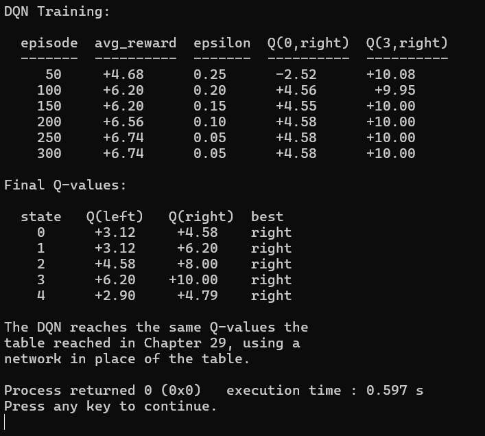
Figure 30-4 has the finished agent learning the same values the table found. The average reward climbs from +4.68 over the first fifty episodes to +6.74 over the last fifty, and the two Q-value columns beside it explain the climb. Q(3, right) reads +10.08 after only fifty episodes and settles to exactly +10.00, which is the correct value, since moving right from state 3 lands on the goal, pays ten, and ends the episode with nothing further to discount. Q(0, right) starts at −2.52, which is not merely imprecise but the wrong sign, and finishes at +4.58, matching to the digit the Bellman value we worked out by hand for the table.
The order in which those two settle is the mechanism made visible. State 3 is adjacent to the reward so its value depends on nothing but the reward itself, and the network gets it almost immediately. State 0 is four steps away and its value depends on state 1, which depends on state 2, which depends on state 3, so the information has to propagate backward through the chain one round of updates at a time. That is the same backward propagation of value we watched in the tabular version, happening here through gradient descent rather than through table assignments.
The final table matches the tabular result across the board, with 4.58, 6.20, 8.00 and 10.00 in the right column and the left column trailing appropriately. State 4 is the exception and it needs saying. It shows Q(left) of +2.90 and Q(right) of +4.79, and both numbers are meaningless, because state 4 is the goal and no action is ever taken from it. A table can simply omit that row, and a network cannot refuse to produce an output, so it emits whatever its weights happen to give for an input it was never trained on. Reading a network’s output for a state it never sees is a mistake that is much easier to make than the equivalent mistake with a table.
The epsilon column shows the decay from 0.25 down to 0.05, and the reward column rises as it falls. Some of that rise is genuine learning and some is simply less exploration, which is the confound we ran into with the table, and separating the two requires evaluating with epsilon set to zero rather than reading the training curve.
30.6 The Path to RLHF
DQN clears the wall the table hit. A network handles a state space of any size, so Atari from raw pixels becomes possible, and the original DQN paper did exactly that on a screen of 84 by 84 pixels, which is a state space of astronomical size that a table could not begin to address.
There is a second wall and DQN does not clear it. The method needs one Q-value per action, computed and compared at every step, which is fine when the action is a joystick with a handful of positions and impossible when the action is a token drawn from a vocabulary of fifty thousand. The output layer alone would need fifty thousand units per state, the argmax would scan all of them at every position, and the network would be spending most of its capacity on values it uses only to discard.
The way around it is to notice what a language model already does. It produces a probability distribution over the whole vocabulary at every position, which is a policy in the sense we defined earlier, so there is no need to add a value estimator on the side. Policy gradient methods adjust that distribution directly using a reward for the completed generation, with no per action values, no argmax over the vocabulary and no target network to maintain.
That is why Chapter 33 builds on the policy gradient work rather than on this chapter. The value based path is the older and better studied half of reinforcement learning, it dominated the field for decades, and it is not the path that produced the aligned models people use. DQN is here because the two fixes in it, replay and the frozen target, recur throughout reinforcement learning in forms that outlast the algorithm they were invented for.
30.7 Key Takeaways
A DQN replaces the Q-table with a network mapping a state to one value per action, so the parameter count depends on the network’s own size rather than on the size of the state space.
The substitution forces a loss where a table needed only an assignment. A table entry can be written directly because nothing else depends on it, and a network has no slot to write to, so every correction reaches the weights through backpropagation and touches all of them.
Consecutive states within an episode are nearly identical, and a network trained on them in order fits a narrow slice of its input and forgets the rest. A table cannot suffer this, since updating state 3 leaves state 0 untouched.
Experience replay stores transitions and draws random batches, which breaks the correlation and lets a rare successful transition contribute to many updates rather than one.
A batch will often contain the same transition twice, which is sampling with replacement rather than a fault, and is the normal result of drawing eight samples from a few dozen.
The Bellman target is computed from the network being trained, so without intervention the target moves with every step. A frozen copy updated every twenty episodes holds it still long enough to be reached.
For a five state problem the network is worse on every measure, at 66 parameters against 10 table entries. The two costs cross as the state space grows, and everything past the crossing belongs to the network.
One-hot input gives up all generalization, since state 3 as [0,0,0,1,0] shares nothing with state 2. That is a table implemented in floating point, and a scaled continuous input is what lets a network notice that nearby states are similar.
The finished DQN reached 4.58, 6.20, 8.00 and 10.00, matching the table exactly, with average reward climbing from +4.68 to +6.74.
Values settle nearest the goal first. Q(3, right) was correct within fifty episodes while Q(0, right) started at −2.52, because the value of state 0 depends on a chain running through every state between it and the reward.
A network cannot decline to answer. It produced Q-values of +2.90 and +4.79 for the terminal state, which are meaningless, where a table would simply have no row.
DQN clears the state space wall and not the action space wall. Fifty thousand tokens means fifty thousand output units and an argmax over all of them at every position, which is why Chapter 33 uses policy gradients on the distribution the model already produces.
30.8 Exercises
Remove the target network (use the policy network for both) and compare training stability. How many episodes before the Q-values diverge or oscillate?
Remove experience replay (train on each transition immediately). Does performance degrade? Why?
Increase the grid to 10 states. The Q-network should generalize: states near the goal should have similar Q-values without visiting every state.
Replace the one-hot state encoding with a single float (state / N_STATES). The network now receives a continuous input. Does it still learn?
Implement double DQN: use the policy network to select the best action, but use the target network to evaluate that action’s Q-value. This reduces overestimation bias.
Count the multiply-accumulate operations per training step for the DQN. Compare to a Q-table update (one addition). At what state space size does the DQN become more efficient than the table?