Activation Functions
Sigmoid, tanh, ReLU, and GELU
3.1 What You Will Learn
In Chapter 2 we used sigmoid as our only activation function. It worked, but sigmoid has problems that show up in deeper networks. In this chapter we build up a library of activation functions, implement each one with its derivative, and see firsthand why modern networks use ReLU and its variants instead of sigmoid. By the end you will have a reusable activation module in C that you can drop into any network.
3.2 Why Activation Functions Matter
Without an activation function, a neuron just computes z = w*x + b. If you can recall, that’s just the formula for a straight line. Straight lines can’t do more than create straight lines, if we stack two straight lines we get another straight line. If we stack a hundred of them, you still get a straight line. It does not matter how many layers you add; the whole network collapses into one layer mathematically, in fact you could replace the entire thing with a single multiplication and an addition. What an activation function does is it breaks the linearity. It bends the output, and that bending is what lets the network learn curves, boundaries, and patterns that a straight line cannot represent. Without it, no amount of depth helps, and with it, each layer can shape the data a little more, and deep networks become genuinely more powerful than shallow ones.
I know we only talked about the step function and sigmoid, but you should know that there are others and not all activation functions behave the same way though. Some train faster than others. Some let gradients flow cleanly through many layers, while others choke them off. The choice matters, and it matters more as networks get deeper. Let us look at each option.
3.3 Sigmoid Review
Although we’re been using sigmoids up to this point, let us revisit it and look more carefully at its behavior, especially at extreme values. Create the following C program.
/* 013_Sigmoid_Review.c */
#include <stdio.h>
#include <math.h>

static float sigmoid(float z)
{
    return 1.0f / (1.0f + expf(-z));
}

static float sigmoid_derivative(float sig_output)
{
    /* Derivative computed from the output, not from z
        */
    return sig_output * (1.0f - sig_output);
}

int main(void)
{
    float values[] = { -10.0f, -5.0f, -2.0f,
        -1.0f, 0.0f,
                        1.0f, 2.0f, 5.0f, 10.0f };
    int n = sizeof(values) / sizeof(values[0]);
    int i;

    printf("  z        sigmoid    derivative\n");
    printf("  -------  ---------  ----------\n");
    for (i = 0; i < n; i++) {
        float s = sigmoid(values[i]);
        float d = sigmoid_derivative(s);
        printf("  %6.1f   %9.6f  %10.6f\n", values[i],
            s, d);
    }
    return 0;
}
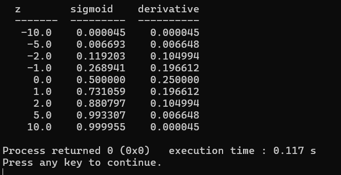
Now that we have the output in Figure 3-1, I want you to look at the derivative column. At z = 0, the derivative peaks at 0.25. By z = 5, it has dropped to 0.006. By z = 10, it is 0.00004, and if you follow that column down you can see for yourself what is happening, which is that the derivative is vanishing.
This is called the vanishing gradient problem and in a deep network, gradients are multiplied together layer by layer during backpropagation. If each layer’s sigmoid derivative is 0.25 at best, then after 10 layers the gradient has been multiplied by 0.25 ten times: 0.25^10 = 0.000001. What this means is that the early layers get almost no gradient signal and when that happens, they stop learning. The sigmoid activation also has a second problem: its output is always positive (between 0 and 1), what this means is that the gradients flowing to the weights are always the same sign for a given sample, which can cause the weights to zigzag during training instead of moving directly toward the optimum.
Don’t worry, in the next section we’ll see how we can improve these problems with tanh.
3.4 Tanh
So, the next function we will look at is the tanh function. You may have seen tan in trigonometry, in case you need a refresher, it’s the ratio of sine to cosine on a unit circle. Hyperbolic tangent is a different function that borrows the name. Instead of being built from circular functions, it is built from exponentials. The “hyperbolic” comes from its relationship to a hyperbola the same way regular trig functions relate to a circle. For neural networks, the geometry does not matter, all we really care about its shape.
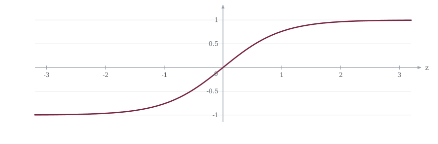
Figure 3-2 has the curve. Tanh looks like a stretched and shifted sigmoid. It maps any input to the range (-1, 1) instead of (0, 1). This means it is centered at zero. When the input is zero, the output is zero. Positive inputs give positive outputs, negative inputs give negative outputs. Sigmoid always outputs a positive number, which can be a problem because it means neuron outputs are always biased in one direction. Tanh does not have that issue.
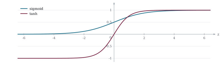
Figure 3-3 sets the two curves against each other. The formula is two exponentials subtracted on top, two exponentials added on the bottom. If you compare it to the sigmoid formula, you can see the family resemblance.
In fact, tanh is just a rescaled sigmoid: tanh(z) = 2 * sigmoid(2z) - 1. They are the same curve, stretched vertically from (0, 1) to (-1, 1) and shifted so zero maps to zero. Like sigmoid, the derivative can be computed from the output itself. If you already computed tanh(z), you do not need z again. Just take the output, square it, and subtract from 1.
The peak derivative is 1.0 when z is zero, compared to 0.25 for sigmoid. That is four times stronger. Gradients travel further through tanh layers before they vanish. It still has the same problem at the extremes though. When z is large positive or large negative, tanh saturates near 1 or −1, the square is near 1, and the derivative drops to nearly zero. The vanishing gradient problem is reduced but not eliminated. We can look at how the tanh function by seeing it first hand in C.
/* 014_Tanh_Activation.c */
#include <stdio.h>
#include <math.h>

static float my_tanh(float z)
{
    /* Guard against overflow for very negative z */
    if (z < -20.0f) return -1.0f;
    float e = expf(-2.0f * z);
    return (1.0f - e) / (1.0f + e);
}

static float tanh_derivative(float tanh_output)
{
    return 1.0f - tanh_output * tanh_output;
}

int main(void)
{
    float values[] = { -10.0f, -5.0f, -2.0f,
        -1.0f, 0.0f,
                        1.0f, 2.0f, 5.0f, 10.0f };
    int n = sizeof(values) / sizeof(values[0]);
    int i;

    printf("  z        tanh       derivative\n");
    printf("  -------  ---------  ----------\n");
    for (i = 0; i < n; i++) {
        float t = my_tanh(values[i]);
        float d = tanh_derivative(t);
        printf("  %6.1f   %9.6f  %10.6f\n", values[i],
            t, d);
    }
    return 0;
}
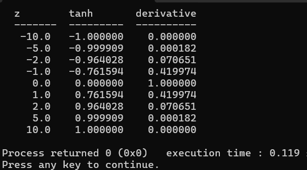
If we look at Figure 3-4, we can see two improvements over sigmoid. Firstly, the peak derivative at z = 0 is 1.0 instead of 0.25. This means the gradients start four times larger. Secondly, the output is centered around zero. This means that positive inputs give positive outputs, negative inputs give negative outputs, so, the hidden layer outputs have a mix of signs, which helps gradient descent converge faster. However, tanh still saturates. At z = 5, the derivative is 0.0002, so our vanishing gradient problem is better than sigmoid but not solved. For very deep networks, we need something that does not saturate.
One thing we added to our function is an overflow guard. When z is very negative, the formula computes expf(-2 * z), which flips the sign and makes a huge positive exponent. Something like z = −50 becomes expf(100), a number far too large for a 32-bit float to hold. The result overflows to infinity, and the division produces garbage. The guard catches this before it happens. If z is below −20, tanh is already −1.0 as far as a float is concerned. There is no point computing the exponential when we already know the answer, so we return −1.0f directly and skip the math that would have blown up.
3.5 ReLU
The Rectified Linear Unit or ReLU is the next activation function we will look at and it is brutally simple, if the input is positive, pass it through unchanged and if it is negative, output zero. There is no exponential, division, or squaring because it is a single comparison.
The max function picks whichever is larger, 0 or z. If z is 3.5, the output is 3.5 and if z is −2.0, the output is 0. There is no curve, squashing or saturation on the positive side. The output grows linearly with the input and on the negative side it is a hard floor at zero. This simplicity is what made deep learning practical, sigmoid and tanh both suffer from vanishing gradients because their derivatives shrink toward zero at the extremes. ReLU has no such problem on the positive side. The derivative is 1 for any positive input, so gradients pass through unchanged no matter how large z gets.
ReLU'(z) = 1   if z > 0
ReLU'(z) = 0   if z < 0
On the negative side the derivative is zero, which means those neurons stop learning entirely. If a neuron gets stuck in the negative zone for every input in the training set, it will never recover. This is called the “dying ReLU” problem and we will address it shortly with Leaky ReLU. In practice enough neurons stay positive to keep the network moving. At z = 0 the derivative is technically undefined because the function has a sharp corner there. In practice we just pick 0 or 1. It does not matter because z landing on exactly 0.000000 with continuous inputs is essentially impossible.
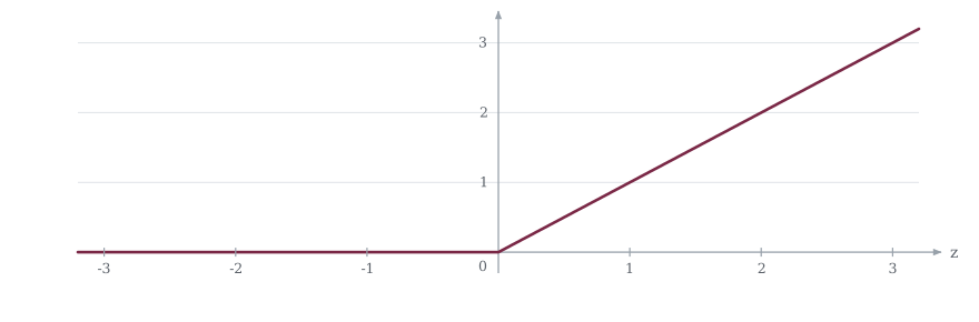
Figure 3-5 plots it. ReLU also computes fast. On an embedded target for example, expf might take dozens of clock cycles and a comparison and a branch take one or two. When you have thousands of neurons running millions of times, that difference adds up. What really stands out to me with this function is its simplicity. It’s literally a pass through, since it does nothing to positive values. It just hands them forward untouched where every other activation function warps the signal in some way. Sigmoid squashes it, tanh squashes it, so they both bend and compress. ReLU on the positive side is literally a wire, very simple, and that turned out to be exactly what deep networks needed. Let’s implement a ReLU activation function in C and examine the results.
/* 015_Relu_Activation.c */
#include <stdio.h>

static float relu(float z)
{
    return z > 0.0f ? z : 0.0f;
}

static float relu_derivative(float z)
{
    return z > 0.0f ? 1.0f : 0.0f;
}

int main(void)
{
    float values[] = { -10.0f, -5.0f, -2.0f,
        -1.0f, 0.0f,
                        1.0f, 2.0f, 5.0f, 10.0f };
    int n = sizeof(values) / sizeof(values[0]);
    int i;

    printf("  z        relu       derivative\n");
    printf("  -------  ---------  ----------\n");
    for (i = 0; i < n; i++) {
        float r = relu(values[i]);
        float d = relu_derivative(values[i]);
        printf("  %6.1f   %9.6f  %10.6f\n", values[i],
            r, d);
    }
    return 0;
}
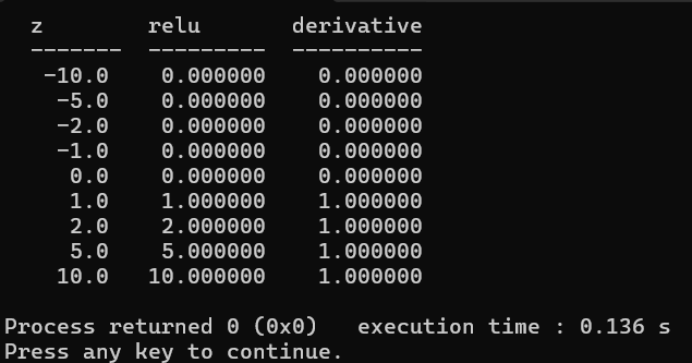
Look at the derivative column in Figure 3-6 for positive z. It is 1, in fact it’s always 1. No matter how deep the network or how large z is, the gradient passes through unchanged. The vanishing gradient problem is gone for positive activations. This is why ReLU transformed deep learning. Before ReLU, training networks deeper than a few layers was painfully slow, however with ReLU, networks with dozens or hundreds of layers became trainable. ReLU has its own problem though a property we call dead neurons as I briefly mentioned in an earlier section. If a neuron’s z goes negative for all inputs in the training set, its output is always zero, its gradient is always zero, and it never recovers. That neuron is said to be dead because it contributes nothing and wastes parameters.
I also want you to notice that ReLU’s derivative needs the input z, not the output. For sigmoid and tanh we could compute the derivative from the output alone. For ReLU we need to know whether z was positive or negative and in practice we just check whether the output is positive, which is the same test.
3.6 GELU
The Gaussian Error Linear Unit is what modern transformers use, including GPT, BERT, and their descendants. It behaves like ReLU in that positive values mostly pass through and negative values get suppressed, but it does so with a smooth curve instead of a hard corner at zero.
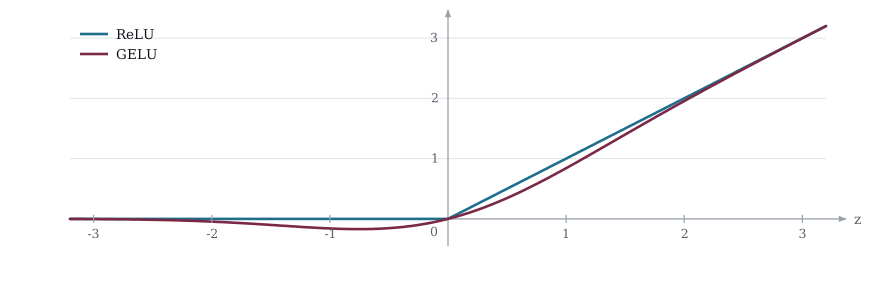
Figure 3-7 sets GELU against ReLU. The name comes from the Gaussian error function, which is related to the normal distribution from statistics. The idea is that instead of cutting off negative values completely like ReLU does, GELU weights each value by the probability that it would be “kept” under a Gaussian distribution. Large positive values have a high probability of being kept so they pass through almost unchanged. Large negative values have a low probability so they get pushed toward zero. Values near zero get partially scaled, which creates a smooth transition instead of the sharp kink that ReLU has. The exact formula uses the error function erf, which is expensive to compute, so in practice everyone uses this polynomial approximation.
GELU(z) = 0.5 * z * (1 + tanh(sqrt(2/pi) * (z + 0.044715 * z^3)))It looks complicated but the implementation is straightforward. The 0.044715 * z^3 term is a curve-fitting constant that makes the approximation accurate to several decimal places. The sqrt(2/pi) is just a fixed number, roughly 0.7978. The whole thing boils down to a few multiplies and one tanh call.
The smooth curve means there are no dead neurons. In ReLU, once a neuron goes negative it is completely off and no gradient flows through it. In GELU, slightly negative inputs still produce a small nonzero output, so a small gradient still flows and the neuron can recover during training. This matters in deep transformers where a dead neuron in an early layer is lost for the rest of training. The derivative is messier to write out analytically, so in practice we use the numerical approach or apply the chain rule through the approximation. For this chapter we will compute it numerically to keep things clear.
/* 016_GELU.c */
#include <stdio.h>
#include <math.h>

static float gelu(float z)
{
    /* Approximation used in GPT and BERT */
    float c = 0.7978845608f;  /* sqrt(2/pi) */
    float inner = c * (z + 0.044715f * z * z * z);
    return 0.5f * z * (1.0f + tanhf(inner));
}

static float gelu_derivative_numerical(float z)
{
    float h = 0.0001f;
    return (gelu(z + h) - gelu(z - h)) / (2.0f * h);
}

int main(void)
{
    float values[] = { -10.0f, -5.0f, -2.0f,
        -1.0f, 0.0f,
                        1.0f, 2.0f, 5.0f, 10.0f };
    int n = sizeof(values) / sizeof(values[0]);
    int i;

    printf("  z        gelu       "
           "derivative\n");
    printf("  -------  ---------  ----------\n");
    for (i = 0; i < n; i++) {
        float g = gelu(values[i]);
        float d = gelu_derivative_numerical(values[i]);
        printf("  %6.1f   %9.6f  %10.6f\n", values[i],
            g, d);
    }
    return 0;
}
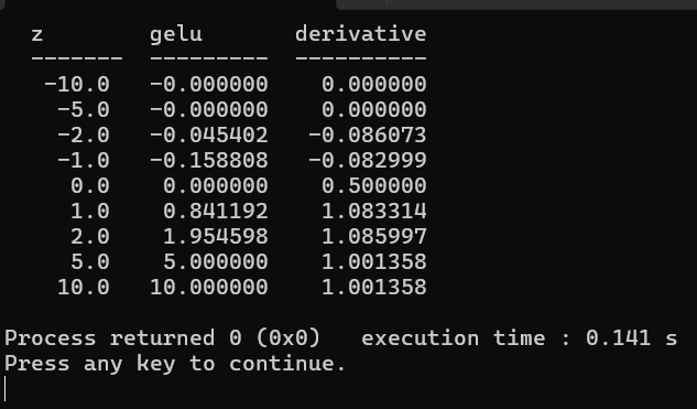
Figure 3-8 has the numbers. GELU behaves like ReLU for positive z (roughly linear with slope near 1) but instead of hard zeroing negative z, it smoothly curves to zero. Very negative values still produce near-zero output, but the transition is gradual. This means there is always a small gradient, so neurons never fully die. You will not use GELU until we get to transformers in later chapters. We introduce it now so you see the full landscape and understand why the field moved from sigmoid to tanh to ReLU to GELU over three decades.
3.7 All Four Side by Side
Let us put all four activation functions in one program so you can see them together and compare their behavior across the same range of inputs.
/* 017_Comparison.c */
#include <stdio.h>
#include <math.h>

static float sigmoid(float z)
{
    return 1.0f / (1.0f + expf(-z));
}
static float sigmoid_d(float z)
{
    float s = sigmoid(z);
    return s * (1.0f - s);
}

static float my_tanh(float z)
{
    if (z < -20.0f) return -1.0f;
    float e = expf(-2.0f*z);
    return (1.0f-e)/(1.0f+e);
}
static float tanh_d(float z)
{
    float t = my_tanh(z);
    return 1.0f - t * t;
}

static float relu(float z)
{
    return z > 0.0f ? z : 0.0f;
}
static float relu_d(float z)
{
    return z > 0.0f ? 1.0f : 0.0f;
}

static float gelu(float z)
{
    float c = 0.7978845608f;
    return 0.5f*z*(1.0f+tanhf(c*(z+0.044715f*z*z*z)));
}
static float gelu_d(float z)
{
    float h = 0.0001f;
    return (gelu(z+h)-gelu(z-h))/(2.0f*h);
}

int main(void)
{
    float values[] = { -3.0f, -2.0f, -1.0f,
        -0.5f, 0.0f,
                        0.5f, 1.0f, 2.0f, 3.0f };
    int n = sizeof(values) / sizeof(values[0]);
    int i;

    printf("--- Output values ---\n");
    printf("  z      sigmoid   tanh"
           "      relu      gelu\n");
    for (i = 0; i < n; i++) {
        float z = values[i];
        printf("  %5.1f  %7.4f"
               "   %7.4f   %7.4f   %7.4f\n",
               z, sigmoid(z), my_tanh(z),
               relu(z), gelu(z));
    }

    printf("\n--- Derivatives ---\n");
    printf("  z      sigmoid   tanh"
           "      relu      gelu\n");
    for (i = 0; i < n; i++) {
        float z = values[i];
        printf("  %5.1f  %7.4f"
               "   %7.4f   %7.4f   %7.4f\n",
               z, sigmoid_d(z), tanh_d(z),
               relu_d(z), gelu_d(z));
    }

    return 0;
}
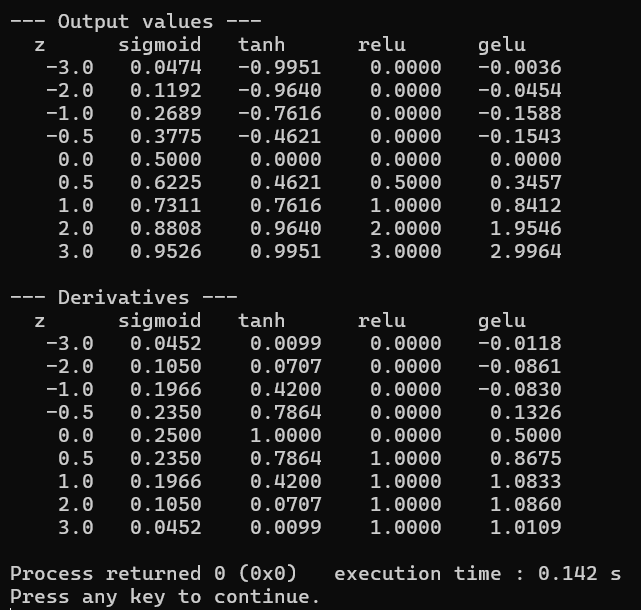
Study the derivative table in Figure 3-9, which runs all four over the same range of z. Sigmoid peaks at 0.25. Tanh peaks at 1.0. ReLU is either 0 or 1 with no in-between. GELU is smooth everywhere and reaches above 1.0 briefly near z = 0.5 before settling to 1.0 for large z.
3.8 Plugging Into the XOR Network
Let us take our XOR network from Chapter 2 and swap the activation function so we can see the difference adding this activation function makes. C is useful for this as we can make the activation a function pointer so we can switch between them easily. This is the kind of modularity you build once and reuse forever as you build up your AI toolbox.
/* 018_XOR_Comparisons.c */
#include <stdio.h>
#include <stdlib.h>
#include <math.h>

/* --- Activation functions and their derivatives --- */

static float act_sigmoid(float z)
{
    return 1.0f / (1.0f + expf(-z));
}
static float der_sigmoid(float z, float out) {
    (void)z;
    return out * (1.0f - out);
}

static float act_tanh(float z) {
    if (z < -20.0f) return -1.0f;
    float e = expf(-2.0f * z);
    return (1.0f - e) / (1.0f + e);
}
static float der_tanh(float z, float out) {
    (void)z;
    return 1.0f - out * out;
}

static float act_relu(float z)
{
    return z > 0.0f ? z : 0.0f;
}
static float der_relu(float z, float out) {
    (void)out;
    return z > 0.0f ? 1.0f : 0.0f;
}

/* --- Network --- */

typedef struct {
    float wh[2][2], bh[2];
    float wo[2], bo;
} Net;

typedef float (*act_fn)(float);
typedef float (*der_fn)(float, float);

static float forward(const Net *n, const float x[2],
    float h[2],
                     float zh[2], float *zo, act_fn act)
{
    int i, j;
    for (i = 0; i < 2; i++) {
        zh[i] = n->bh[i];
        for (j = 0; j < 2; j++)
            zh[i] += n->wh[i][j] * x[j];
        h[i] = act(zh[i]);
    }
    *zo = n->bo;
    for (i = 0; i < 2; i++)
        *zo += n->wo[i] * h[i];
    return act(*zo);
}

static void backward(Net *n, const float x[2],
    const float h[2],
                     const float zh[2], float zo,
                     float y, float t, float lr,
                     der_fn der)
{
    int i, j;
    float delta_out = -2.0f * (t - y) * der(zo, y);
    float delta_h[2];

    for (i = 0; i < 2; i++)
        delta_h[i] = delta_out * n->wo[i] * der(zh[i],
            h[i]);

    for (i = 0; i < 2; i++)
        n->wo[i] -= lr * delta_out * h[i];
    n->bo -= lr * delta_out;

    for (i = 0; i < 2; i++) {
        for (j = 0; j < 2; j++)
            n->wh[i][j] -= lr * delta_h[i] * x[j];
        n->bh[i] -= lr * delta_h[i];
    }
}

static void init_random(Net *n)
{
    int i, j;
    for (i = 0; i < 2; i++) {
        for (j = 0; j < 2; j++)
            n->wh[i][j] = ((float)rand() / RAND_MAX)
                * 2.0f - 1.0f;
        n->bh[i] = ((float)rand() / RAND_MAX) * 2.0f
            - 1.0f;
        n->wo[i] = ((float)rand() / RAND_MAX) * 2.0f
            - 1.0f;
    }
    n->bo = ((float)rand() / RAND_MAX) * 2.0f - 1.0f;
}

static void train_xor(const char *name, act_fn act,
    der_fn der)
{
    float X[4][2] = { {0, 0}, {0, 1}, {1, 0}, {1, 1} };
    float T[4] = { 0, 1, 1, 0 };
    Net net;
    float lr = 1.0f;
    int epoch, s;

    srand(42);
    init_random(&net);

    for (epoch = 0; epoch < 10000; epoch++) {
        float total_loss = 0.0f;
        for (s = 0; s < 4; s++) {
            float h[2], zh[2], zo, y, diff;
            y = forward(&net, X[s], h, zh, &zo, act);
            diff = T[s] - y;
            total_loss += diff * diff;
            backward(&net, X[s], h, zh, zo, y, T[s], lr,
                der);
        }
        if (epoch == 9999)
            printf("%-8s  final loss=%.6f  ", name,
                total_loss / 4.0f);
    }

    /* Final check */
    for (s = 0; s < 4; s++) {
        float h[2], zh[2], zo;
        float y = forward(&net, X[s], h, zh, &zo, act);
        printf("%.2f ", y);
    }
    printf("\n");
}

int main(void)
{
    printf("Activation  Final Loss"
           "    Outputs (00 01 10 11)\n");
    printf("-------------------------"
           "--------------------------\n");
    train_xor("sigmoid", act_sigmoid, der_sigmoid);
    train_xor("tanh",    act_tanh,    der_tanh);
    train_xor("relu",    act_relu,    der_relu);
    return 0;
}
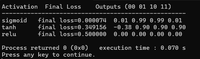
Figure 3-10 trains the same XOR network four times, one activation each. With seed 42 and a learning rate of 1.0, sigmoid nails it but tanh gets stuck in a local minimum where it outputs high for three of the four cases. ReLU fails completely because both hidden neurons landed in the negative region for all inputs and died, giving zero output together with zero gradient, and no path to recovery. That is the dead neuron problem we were talking about earlier playing out on a tiny network.
These results depend on the random seed and learning rate though. Try seed 7 or seed 100 and you will get different winners. The point is not that one activation is always better on XOR, it is that each activation has characteristic failure modes you need to understand. Sigmoid vanishes, tanh can get stuck, and ReLU can die. On larger problems with hundreds of neurons the dead neuron problem is less catastrophic because not every neuron dies at once, and ReLU’s gradient advantages outweigh the occasional losses, “economies of scale” as they say.
One design change worth noting in the code is the derivative function now takes both z (the pre-activation value) and out (the activation output). Sigmoid and tanh only need out to compute their derivatives while ReLU only needs z. By passing both, one function signature works for all three activations and the unused argument gets cast to void so the compiler does not warn about it.
3.9 When to Use What
Here is the practical guide in a nutshell that will serve you as you start doing your own experiments.
Sigmoid. Almost never in hidden layers. Still used as the output activation for binary classification (is this a cat or not?) because it produces a value between 0 and 1 that can be interpreted as a probability.
Tanh. Occasionally in hidden layers of RNNs and LSTMs (if you never used those don’t worry we have more on those later), where the output range of (-1, 1) is useful for gating. We will see this in Chapters 15 and 16, but rarely used elsewhere.
ReLU. The default for hidden layers in feedforward and convolutional networks. Fast to compute (one comparison), strong gradients, works well in practice. Use this unless you have a reason not to.
GELU. The default for transformer architectures. Smoother than ReLU, because it has no dead neurons, which makes it slightly better performance on language and vision tasks. However, it’s more expensive to compute than ReLU because of the tanh and cubic terms, but the cost is negligible compared to the matrix multiplications in a transformer. Once you have the compute this may be worth doing in a modern architecture.
For our purposes going forward, we will use ReLU in Chapters 4-9 for feedforward and convolutional networks, tanh inside LSTMs and GRUs in Chapters 15-16, and GELU when we build transformers starting in Chapter 24 so you’ll get exposure to all.
3.10 Key Takeaways
Activation functions add non-linearity. Without them, a deep network collapses to a single layer.
Sigmoid saturates at both ends. Its peak derivative is only 0.25. This causes vanishing gradients in deep networks.
Tanh is centered at zero with a peak derivative of 1.0. Better than sigmoid, but still saturates.
ReLU passes positive values unchanged (derivative = 1) and zeros out negative values (derivative = 0). No saturation for positive inputs, but dead neurons are possible.
GELU is a smooth approximation to ReLU used in transformers. No dead neurons, slightly better empirical performance.
The derivative function signature float der(float z, float out) covers all activations. Sigmoid and tanh use out. ReLU uses z. Pass both, ignore what you do not need.
3.11 Exercises
Implement Leaky ReLU. f(z) = z if z > 0, else 0.01 * z. How does it solve the dead neuron problem? Train XOR with it.
Implement the exact sigmoid derivative from z (not from the output) and verify it produces the same numbers. Why is the output-based version preferred?
Stack 5 hidden layers of 4 neurons each with sigmoid activation. Train on XOR. Then swap to ReLU. Compare how many epochs each needs. This is the vanishing gradient problem made visible.
Add GELU to the 018_XOR_Comparisons.c comparison. You will need a numerical derivative in the backward pass (use the central difference formula from 016_GELU.c). How does it compare to the others on XOR?
Plot (on paper or with a plotting tool) all four activation functions and their derivatives on the range [−5, 5]. The shape tells you everything about why one works better than another.
Read the ReLU implementation in KANN (kautodiff.c, search for kad_op_relu). It is five lines. Compare it to yours. What is the same? What is different?