Loss Functions
MSE, cross-entropy, and softmax
4.1 What You Will Learn
In Chapter 2 we used mean squared error to measure how wrong our network was. It worked for XOR, but MSE is not always the right choice. In this chapter we build three loss functions from scratch, understand when to use each one, and see how the choice of loss function changes the gradients that flow through the network during training.
4.2 What a Loss Function Does
A loss function takes what the network predicted and what the correct answer was, and turns the pair into a single number where lower means better. Training is the process of adjusting weights until that number is as small as we can get it. Scoring is the obvious job and it is not the important one, because the number by itself only tells us how badly we are doing and never what to do about it. The derivative is what tells the network which direction to push its outputs, and that is the part every loss function in this chapter exists to provide.
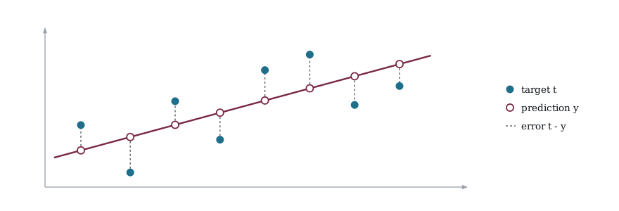
Figure 4-1 shows the shape of the idea with a handful of predictions. Each target sits somewhere, each prediction sits somewhere else, and the gap between them is the error on that one example. A loss function is a rule for collapsing all of those gaps into one number, and the rule you choose decides which gaps get taken seriously. Squaring them makes a single large gap dominate the total, while other rules spread the blame more evenly, so two networks trained on identical data with different losses will not converge to the same weights.
Different losses also push differently once training starts. MSE pushes gently when the prediction is close and hard when it is far off, which sounds reasonable and turns out to be exactly wrong for classification. Cross-entropy pushes hardest when the prediction is confident and wrong, which is the moment correction is worth the most. We build each one and watch the difference show up in the gradients.
4.3 Mean Squared Error
We used MSE in Chapter 2 so let us look at it more carefully. For a single prediction y and target t, the loss is the difference between them, squared.
If y is 0.9 and t is 1.0, the error is 0.1 and the loss is 0.01. If y is 0.5 and t is 1.0, the error is 0.5 and the loss is 0.25. Being off by five times as much produces twenty-five times the loss, not five times, which is of course what squaring does. For N samples we average the individual losses so the total does not grow just because we have more training data.
With our XOR problem N is 4, so we sum the squared errors for all four input pairs and divide by 4. Whether you train on 4 samples or 4000, the MSE stays on a comparable scale and the learning rate does not need to change. The derivative with respect to y tells us which direction to push the prediction and by how much.
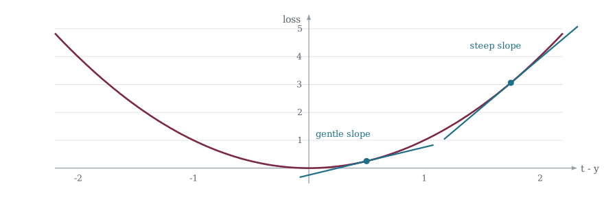
The parabola in Figure 4-2 is why MSE behaves the way it does. The height of the curve is the loss and the steepness is the gradient, so a prediction that is already close sits near the bottom where the curve is almost flat and the correction is small, while a prediction that is far out sits on a steep section and gets pushed hard. For a regression problem that is the behavior we want, since an answer that is nearly right should be left nearly alone.
If y is too low the result is negative, meaning we need to increase y. If y is too high the result is positive, meaning we need to decrease y. The further off the prediction is, the larger this value gets, so the network naturally takes bigger corrective steps for bigger mistakes and smaller steps as it gets closer to the target.
/* 019_MSE_Review.c */
#include <stdio.h>

static float mse_loss(float y, float t)
{
    float diff = t - y;
    return diff * diff;
}

static float mse_derivative(float y, float t)
{
    return -2.0f * (t - y);
}

int main(void)
{
    float targets[] = { 0.0f, 1.0f, 1.0f, 0.0f }; /* XOR */
    /* close predictions */
    float good[] = { 0.05f, 0.92f, 0.95f, 0.08f };
    /* poor predictions */
    float bad[]  = { 0.80f, 0.20f, 0.30f, 0.70f };
    int i;

    printf("--- Good predictions ---\n");
    printf("  target  predict   loss      gradient\n");
    float total_good = 0.0f;
    for (i = 0; i < 4; i++) {
        float l = mse_loss(good[i], targets[i]);
        float g = mse_derivative(good[i], targets[i]);
        total_good += l;
        printf("  %.2f    %.2f     %.4f    %+.4f\n",
               targets[i], good[i], l, g);
    }
    printf("  MSE = %.4f\n", total_good / 4.0f);

    printf("\n--- Bad predictions ---\n");
    printf("  target  predict   loss      gradient\n");
    float total_bad = 0.0f;
    for (i = 0; i < 4; i++) {
        float l = mse_loss(bad[i], targets[i]);
        float g = mse_derivative(bad[i], targets[i]);
        total_bad += l;
        printf("  %.2f    %.2f     %.4f    %+.4f\n",
               targets[i], bad[i], l, g);
    }
    printf("  MSE = %.4f\n", total_bad / 4.0f);

    return 0;
}
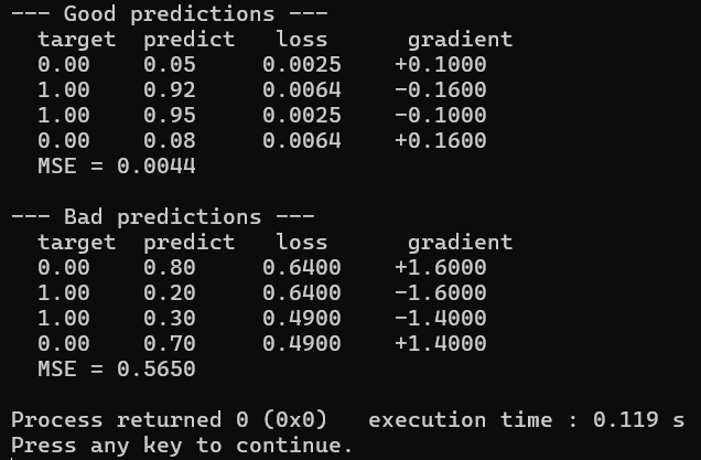
Look at the gradient column in Figure 4-3, which covers good predictions and bad ones alike. For good predictions the gradient is small (the network is close, small nudges are enough). For bad predictions the gradient is large (the network is far off, it needs a big correction). The sign carries the direction, so that a positive gradient means push y down while a negative one means push y up.
MSE works well for regression problems where the output is a continuous value (predicting a temperature, a voltage, a distance). For classification problems (is this a 0 or a 1?), there is a better option.
4.4 The Problem with MSE for Classification
Consider a network with a sigmoid output trying to classify something as class 1, so the target is 1.0. What happens when the network predicts 0.0001?
With MSE the loss is (1 - 0.0001)^2 which comes out to 0.9998. The gradient is −2 * (1 - 0.0001) which is −1.9998 (this comes from the MSE derivative formula, this is the constant that falls out of differentiating the square). That sounds like a strong correction signal, but there is a problem hiding behind the sigmoid. The gradient has to pass through the sigmoid derivative before it reaches the weights, and when the sigmoid output is 0.0001 the sigmoid derivative is 0.0001 * (1 - 0.0001) which is 0.00009999. That MSE gradient of nearly −2.0 gets multiplied by 0.0001 and almost nothing reaches the weights.
So, you end up in a situation where the network is confidently wrong, the loss is nearly as high as it can get, but the gradient is too small to fix it. The loss function is screaming that the prediction is terrible but the sigmoid is choking the signal before it arrives anywhere useful. Training stalls and the weights barely move even though they desperately need to. This is not a hypothetical problem, it happens in practice any time you pair MSE with a sigmoid output on a classification task. Let us see this in C.
/* 020_MSE_Problem.c */
#include <stdio.h>
#include <math.h>

static float sigmoid(float z)
{
    return 1.0f / (1.0f + expf(-z));
}

int main(void)
{
    /* Simulate the gradient that reaches a weight */
    float predictions[] =
        { 0.0001f, 0.01f, 0.1f, 0.5f, 0.9f };
    float target = 1.0f;
    int i;

    printf("MSE gradient through sigmoid (target=1.0):\n");
    printf("  predict  mse_grad  sig_deriv  eff\n");
    for (i = 0; i < 5; i++) {
        float y = predictions[i];
        float mse_grad  = -2.0f * (target - y);
        float sig_deriv = y * (1.0f - y);
        float effective = mse_grad * sig_deriv;
        printf("  %.4f    %+7.4f    %.6f   %+.6f\n",
               y, mse_grad, sig_deriv, effective);
    }

    return 0;
}
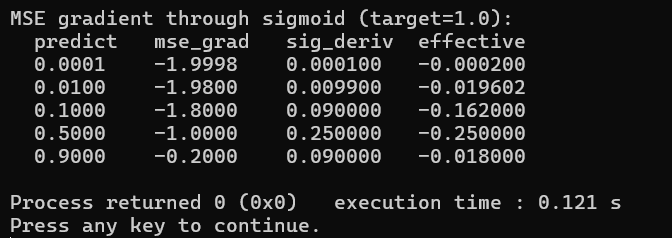
Figure 4-4 puts the same gradient through the sigmoid derivative. The effective gradient column shows the problem., when the prediction is 0.0001 (very wrong), the effective gradient is tiny because the sigmoid derivative is near zero. When the prediction is 0.5 (moderately wrong), the effective gradient is strongest. MSE with sigmoid produces the largest gradients when the network is half-right, not when it is most wrong, that is backwards for classification. This is a problem.
However, the solution to this problem is something called binary cross-entropy which we will look at in the next section.
4.5 Binary Cross-Entropy
Binary cross-entropy fixes this problem with a rather clever solution. Instead of squaring the error, it uses logarithms, and that changes everything. We can take a closer look at logs to understand what’s going on. A logarithm simply asks the question, “what power do I raise this base to, to get that number?”. So, log base 10 of 1000 is 3, because 10^3 = 1000. In software and neural networks, log means the natural logarithm (base e, roughly 2.718) but the intuition is the same. The property that matters here is what log does to the numbers between 0 and 1, because that’s where probabilities live. Log(1.0) = 0, log (0.5) is about −0.69, log(0.01) is about −4.6. log(0.0001) is about −9.2, As the input gets closer to zero, log shoots toward negative infinity. That curve is the entire reason cross entropy works.
With mean squared error, if the network outputs 0.99 when the answer is 1.0, the error is (1.0 - 0.99)^2 = 0.0001. If the network outputs 0.01 when the answer is 1.0, the error is (1.0 - 0.01)^2 = 0.98. That’s a ratio of about 10,000x between “almost right” and “completely wrong.” Sounds like a lot, but the gradient (the learning signal) flattens out at the extremes because of how sigmoid squashes things which of course means the network gets lazy near the edges.
Log fixes the problem. Cross-entropy uses -log(y) when the target is 1. If the network outputs 0.99, the loss is -log(0.99) = 0.01. If it outputs 0.01, the loss is -log(0.01) = 4.6. If it outputs 0.0001, the loss is -log(0.0001) = 9.2. The punishment doesn’t just grow, it accelerates. A confident wrong answer gets hammered exponentially harder than a mildly wrong one. The gradient stays strong exactly where the network needs the biggest correction.
The formula has two cases in it, written here for a single prediction y and a target t that both sit between 0 and 1.
This looks more complicated than MSE but it breaks into two simple cases. When t is 1, the second term (1-t) disappears because (1 - t) is zero, and you are left with -log(y). The network is punished based on how far y is from 1. An output of 0.99 costs almost nothing, while an output of 0.01 costs a great deal. When t is 0, the first term disappears because t is zero, and you are left with -log(1 - y). So, the loss function only cares about one side at a time. how close is y to the correct answer?
The logarithm is very powerful. Think about this if y is 0.9 and the target is 1, -log(0.9) is about 0.105, a small loss. If y is 0.5, -log(0.5) is 0.693, a moderate loss. If y is 0.0001, -log(0.0001) is 9.21. The punishment grows explosively as the prediction moves away from the target. Thus the network cannot be confidently wrong without paying an enormous price for it.
The derivative is where the real advantage shows up.
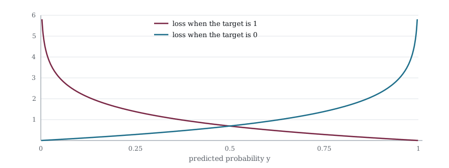
Figure 4-5 shows why this loss suits classification. Only one of the two curves applies to any given example, chosen by whether the target is 1 or 0, and each one falls to zero when the prediction agrees with the target and climbs without bound as the prediction moves away. Being confidently wrong costs far more than being merely uncertain, which is the property MSE lacks, and it is why a network trained with cross-entropy escapes a bad start much faster than the same network trained with squared error.
When the prediction is very wrong, say y is near 0 and the target is 1, the gradient is -t/y which is −1/0.0001 or −10000. Compare that to MSE where the gradient was −2 but got choked to almost nothing by the sigmoid derivative. With BCE the gradient explodes in the right direction, overwhelming the sigmoid’s vanishing derivative and forcing the weights to move.
There is a numerical trap though. The log of 0 is negative infinity, and if y ever hits exactly 0 or exactly 1 the program crashes. We need to clamp y away from the extremes. A floor of 1e-9 is standard practice. If y falls below 0.000000001 we just call it 0.000000001, close enough to zero for the math to work but far enough away that the logarithm does not explode.
/* 021_BCE.c */
#include <stdio.h>
#include <math.h>

static float bce_loss(float y, float t)
{
    /* Clamp to avoid log(0) */
    float tiny = 1e-9f;
    if (y < tiny) y = tiny;
    if (y > 1.0f - tiny) y = 1.0f - tiny;

    return -(t * logf(y) + (1.0f - t) * logf(1.0f - y));
}

static float bce_derivative(float y, float t)
{
    float tiny = 1e-9f;
    if (y < tiny) y = tiny;
    if (y > 1.0f - tiny) y = 1.0f - tiny;

    return -(t / y) + (1.0f - t) / (1.0f - y);
}

int main(void)
{
    float predictions[] =
        { 0.0001f, 0.01f, 0.1f, 0.5f, 0.9f, 0.99f };
    float target = 1.0f;
    int i, n = 6;

    printf("BCE loss and gradient (target=1.0):\n");
    printf("  predict   loss      gradient\n");
    for (i = 0; i < n; i++) {
        float l = bce_loss(predictions[i], target);
        float g = bce_derivative(predictions[i], target);
        printf("  %.4f    %7.4f   %+10.4f\n",
               predictions[i], l, g);
    }

    return 0;
}
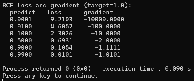
Figure 4-6 walks the prediction toward the target and reports the loss and the gradient at each stop. Compare the gradient column to the MSE version. When the prediction is 0.0001 (very wrong), BCE’s gradient is enormous. It screams at the network to fix itself. As the prediction approaches 1.0 (correct), the gradient shrinks to nearly zero. This is exactly the right behavior for classification.
4.6 BCE vs MSE Through Sigmoid
Now let us compare what actually reaches the weights after passing through the sigmoid derivative. This is the comparison that matters for training speed.
/* 022_BCE_VS_MSE.c */
#include <stdio.h>
#include <math.h>

int main(void)
{
    float predictions[] =
        { 0.0001f, 0.01f, 0.1f, 0.5f, 0.9f };
    float target = 1.0f;
    float tiny = 1e-9f;
    int i;

    printf("Effective gradient (target=1.0):\n");
    printf("  predict   MSE*sig'     BCE*sig'\n");
    for (i = 0; i < 5; i++) {
        float y = predictions[i];
        float sig_d = y * (1.0f - y);

        /* MSE effective */
        float mse_g = -2.0f * (target - y);
        float mse_eff = mse_g * sig_d;

        /* BCE effective */
        float yc = y < tiny ? tiny
                   : (y > 1.0f - tiny ? 1.0f - tiny : y);
        float bce_g = -(target / yc)
                      + (1.0f - target) / (1.0f - yc);
        float bce_eff = bce_g * sig_d;

        printf("  %.4f    %+10.6f    %+10.6f\n",
               y, mse_eff, bce_eff);
    }

    return 0;
}
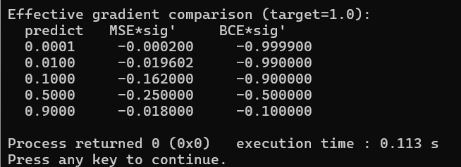
Figure 4-7 sets the two effective gradients side by side. The BCE effective gradient is much larger when the prediction is wrong (y near 0). Something rather elegant happens in the mathematics. the BCE derivative (which has y in the denominator) partially cancels the sigmoid derivative (which has y as a factor). The sigmoid saturation that kills MSE gradients barely affects BCE. This cancellation is not a coincidence. Cross-entropy was designed for sigmoid outputs. They are a natural pair.
This is why binary cross-entropy is the standard loss for binary classification with sigmoid output. Use MSE for regression. Use BCE for classification.
4.7 More Than Two Options
Binary cross-entropy handles “yes or no” decisions, but what if you have more than two classes? A digit recognizer needs to choose between 0, 1, 2, all the way through 9. That is ten classes, and a single sigmoid output cannot represent ten choices. Multi-class problems need two pieces. an output layer that produces a probability distribution across all classes, and a loss function that measures how far that distribution is from the correct answer.
The output layer uses softmax. Given a vector of raw scores, which are called logits, softmax converts them into probabilities that add up to 1.
Each output gets exponentiated, then divided by the sum of all the exponentiated outputs. The exponentiation makes every value positive, and dividing by the sum forces them to add up to 1.0. If one logit is much larger than the others, its softmax output will dominate and be close to 1 while the rest will be close to 0. If all logits are similar, the probabilities will be spread roughly evenly. Essentially it is a competition each class gets a share of the total probability proportional to the exponential of its score. The word “logit” comes up a lot so let us be clear about what it means. The logit is just the raw output of the neuron before any activation function is applied, the weighted sum plus bias. It can be any number, positive or negative, large or small. Softmax takes those raw numbers and turns them into a proper probability distribution.
There is a numerical stability problem though. If any z_i is large, say 500, then exp(500) overflows a 32-bit float. The fix is to subtract the maximum value from all logits before computing the exponential. This does not change the result because the subtraction cancels out in the division.
After subtracting the max, the largest exponent is exp(0) which is 1, and everything else is smaller. No overflow is possible. This is the same kind of numerical guard we saw with the tanh overflow and the BCE log(0) clamp. Floating point math on embedded targets requires this kind of defensive thinking. The max values cancel out which adds a small degree of robustness to our algorithm.
/* 023_Softmax.c */
#include <stdio.h>
#include <math.h>
#include <float.h>

static void softmax(const float *z, float *out, int n)
{
    float max_val, sum;
    int i;

    /* Find max for numerical stability */
    max_val = -FLT_MAX;
    for (i = 0; i < n; i++)
        if (z[i] > max_val) max_val = z[i];

    /* Compute exp(z_i - max) and sum */
    sum = 0.0f;
    for (i = 0; i < n; i++) {
        out[i] = expf(z[i] - max_val);
        sum += out[i];
    }

    /* Normalize */
    for (i = 0; i < n; i++)
        out[i] /= sum;
}

int main(void)
{
    /* Raw logits from a 4-class network */
    float logits[] = { 2.0f, 1.0f, 0.1f, -1.0f };
    float probs[4];
    float sum = 0.0f;
    int i;

    softmax(logits, probs, 4);

    printf("Logits -> Softmax probabilities:\n");
    for (i = 0; i < 4; i++) {
        printf("  class %d: logit=%5.1f  prob=%.4f\n",
               i, logits[i], probs[i]);
        sum += probs[i];
    }
    printf("  Sum of probabilities: %.6f\n", sum);

    /* Test with extreme values */
    printf("\nExtreme logits (stability test):\n");
    float extreme[] = { 500.0f, 499.0f, 498.0f, 0.0f };
    softmax(extreme, probs, 4);
    for (i = 0; i < 4; i++)
        printf("  class %d: logit=%5.0f  prob=%.4f\n",
               i, extreme[i], probs[i]);

    return 0;
}
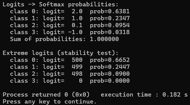
Figure 4-8 turns logits into probabilities and includes the overflow test at 500. The probabilities sum to 1.0. The highest logit gets the highest probability. Even with logits of 500, the subtraction trick prevents overflow. The output is a valid probability distribution.
4.8 Categorical Cross-Entropy
Now we need a loss function for softmax outputs. Categorical cross-entropy (also called multi-class cross-entropy) is the standard.
loss = -sum(t_i * log(p_i))Where t is a one-hot vector (all zeros except a 1 at the correct class) and p is the softmax output. Since t is one-hot, only one term survives.
loss = -log(p_correct)If the network assigns high probability to the correct class, the loss is small. If it assigns low probability, the loss is large. Like BCE, the log means that confident wrong answers are punished severely.
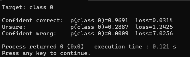
Figure 4-9 runs categorical cross-entropy on a three class example. The loss jumps dramatically from confident-correct to confident-wrong. That steep penalty is what drives the network to be both accurate and calibrated.
4.9 The Softmax-CrossEntropy Gradient
Computing the gradient of cross-entropy through softmax separately is messy. But combined, something beautiful happens. The gradient of the loss with respect to the logits z simplifies neatly.
d_loss/dz_i = p_i - t_iThat is the whole gradient, which comes out as prediction minus target for each class. For the correct class, the gradient is (p - 1), pushing the logit up. For all wrong classes, the gradient is (p - 0) = p, pushing the logits down. The result is simple to implement, numerically stable, and free of the traps that come with computing the two derivatives separately.
This is why softmax and cross-entropy are always used together. The combined gradient is trivially simple and well-behaved. Let us implement it.
/* 024_Cross_Entrophy_Gradient.c */
#include <stdio.h>
#include <math.h>
#include <float.h>

static void softmax(const float *z, float *out, int n)
{
    float max_val = -FLT_MAX, sum = 0.0f;
    int i;
    for (i = 0; i < n; i++)
        if (z[i] > max_val) max_val = z[i];
    for (i = 0; i < n; i++) {
        out[i] = expf(z[i] - max_val);
        sum += out[i];
    }
    for (i = 0; i < n; i++)
        out[i] /= sum;
}

static void softmax_ce_gradient(const float *probs,
                                int target,
                                 float *grad, int n)
{
    int i;
    for (i = 0; i < n; i++)
        grad[i] = probs[i];
    grad[target] -= 1.0f;   /* p_i - t_i, one-hot */
}

int main(void)
{
    float logits[] = { 2.0f, 1.0f, 0.1f, -1.0f };
    float probs[4], grad[4];
    int target = 0;
    int i;

    softmax(logits, probs, 4);
    softmax_ce_gradient(probs, target, grad, 4);

    printf("Target: class %d\n\n", target);
    printf("  class  logit   prob    gradient\n");
    for (i = 0; i < 4; i++)
        printf("  %d      %5.1f   %.4f  %+.4f\n",
               i, logits[i], probs[i], grad[i]);

    printf("\nInterpretation:\n");
    printf("  Class 0 (correct): gradient is"
           " negative -> push logit UP\n");
    printf("  Classes 1-3 (wrong): gradient is"
           " positive -> push logits DOWN\n");

    return 0;
}
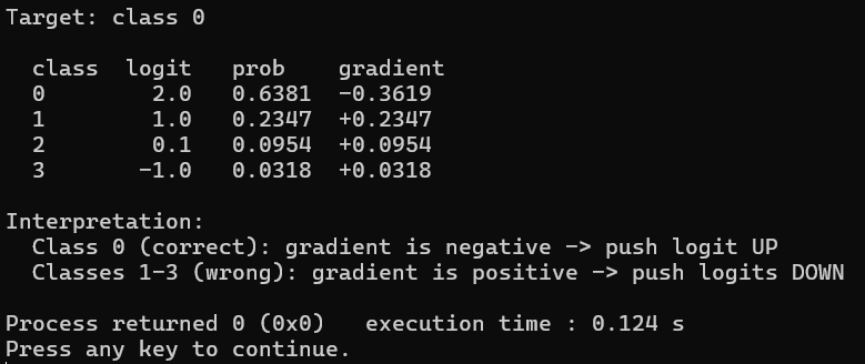
Figure 4-10 pushes one class up and the other three down. The gradient for the correct class is negative (push up). The gradients for wrong classes are positive (push down). The magnitudes are proportional to how much probability each class currently has. Classes with more probability get pushed down harder. The network learns to redistribute probability from wrong classes to the right one.
4.10 Plugging Into a Network
Let us bring it all together. We will train a small network on a classification problem using cross-entropy loss and softmax output, and compare it to the same network trained with MSE. This program is a complete 2 later neural network trained from scratch in pure C. It learns to classify 2D points into 4 quadrants, so the network takes two inputs (x, y, coordinates) and has to work out which quadrant the point is in. (-1,-1) is class 0, (-1,+1) is class 1, (+1,-1) is class 2, (+1,+1) is class 3. We’ll structure the network so that the architecture is 2 inputs, 4 hidden neurons with sigmoid activation, 4 output neurons with softmax. This is small enough to trace every value by hand, big enough to actually learn a nonlinear decision boundary.
/* 025_Train_Compare.c */
#include <stdio.h>
#include <stdlib.h>
#include <math.h>
#include <float.h>

static float sigmoid(float z)
{ return 1.0f / (1.0f + expf(-z)); }

/* 2-input, 4-hidden, 4-output (4-class classification) */
typedef struct {
    float wh[4][2], bh[4];   /* hidden layer */
    float wo[4][4], bo[4];   /* output layer */
} Net;

static void forward(const Net *n, const float x[2],
           float h[4], float logits[4],
           float probs[4])
{
    int i, j;

    /* Hidden layer with sigmoid */
    for (i = 0; i < 4; i++) {
        float z = n->bh[i];
        for (j = 0; j < 2; j++)
            z += n->wh[i][j] * x[j];
        h[i] = sigmoid(z);
    }

    /* Output layer: raw logits */
    for (i = 0; i < 4; i++) {
        logits[i] = n->bo[i];
        for (j = 0; j < 4; j++)
            logits[i] += n->wo[i][j] * h[j];
    }

    /* Softmax */
    {
        float max_val = -FLT_MAX, sum = 0.0f;
        for (i = 0; i < 4; i++)
            if (logits[i] > max_val) max_val = logits[i];
        for (i = 0; i < 4; i++) {
            probs[i] = expf(logits[i] - max_val);
            sum += probs[i];
        }
        for (i = 0; i < 4; i++)
            probs[i] /= sum;
    }
}

static void backward_ce(Net *n,
                        const float x[2], const float h[4],
            const float probs[4],
            int target, float lr)
{
    int i, j;
    float d_out[4], d_h[4];

    /* Output gradient: p - t */
    for (i = 0; i < 4; i++)
        d_out[i] = probs[i];
    d_out[target] -= 1.0f;

    /* Hidden gradient */
    for (i = 0; i < 4; i++) {
        d_h[i] = 0.0f;
        for (j = 0; j < 4; j++)
            d_h[i] += d_out[j] * n->wo[j][i];
        d_h[i] *= h[i] * (1.0f - h[i]);
    }

    /* Update output weights */
    for (i = 0; i < 4; i++) {
        for (j = 0; j < 4; j++)
            n->wo[i][j] -= lr * d_out[i] * h[j];
        n->bo[i] -= lr * d_out[i];
    }

    /* Update hidden weights */
    for (i = 0; i < 4; i++) {
        for (j = 0; j < 2; j++)
            n->wh[i][j] -= lr * d_h[i] * x[j];
        n->bh[i] -= lr * d_h[i];
    }
}

static void init_random(Net *n)
{
    int i, j;
    for (i = 0; i < 4; i++) {
        for (j = 0; j < 2; j++)
            n->wh[i][j] =
                ((float)rand() / RAND_MAX) * 2.0f - 1.0f;
        n->bh[i] = 0.0f;
        for (j = 0; j < 4; j++)
            n->wo[i][j] =
                ((float)rand() / RAND_MAX) * 2.0f - 1.0f;
        n->bo[i] = 0.0f;
    }
}

int main(void)
{
    /* 4 quadrants -> 4 classes */
    float X[4][2]  = { {-1,-1}, {-1, 1}, { 1,-1}, { 1, 1} };
    int targets[4] = {  0,       1,       2,       3      };
    Net net;
    float lr = 0.5f;
    int epoch, s;

    srand(42);
    init_random(&net);

    for (epoch = 0; epoch < 5000; epoch++) {
        float total_loss = 0.0f;
        int correct = 0;

        for (s = 0; s < 4; s++) {
            float h[4], logits[4], probs[4];
            float tiny = 1e-9f;

            forward(&net, X[s], h, logits, probs);

            float p = probs[targets[s]];
            if (p < tiny) p = tiny;
            total_loss += -logf(p);

            /* Check accuracy */
            int pred = 0;
            for (int k = 1; k < 4; k++)
                if (probs[k] > probs[pred]) pred = k;
            if (pred == targets[s]) correct++;

            backward_ce(&net, X[s], h, probs,
                        targets[s], lr);
        }

        if ((epoch + 1) % 1000 == 0)
            printf("epoch %4d  loss=%.4f  accuracy=%d/4\n",
                   epoch + 1, total_loss / 4.0f, correct);
    }

    /* Final predictions */
    printf("\nFinal predictions:\n");
    for (s = 0; s < 4; s++) {
        float h[4], logits[4], probs[4];
        forward(&net, X[s], h, logits, probs);
        printf("  x=(%+.0f,%+.0f)  probs="
               "[%.3f %.3f %.3f %.3f]  target=%d\n",
               X[s][0], X[s][1],
               probs[0], probs[1],
               probs[2], probs[3],
               targets[s]);
    }

    return 0;
}
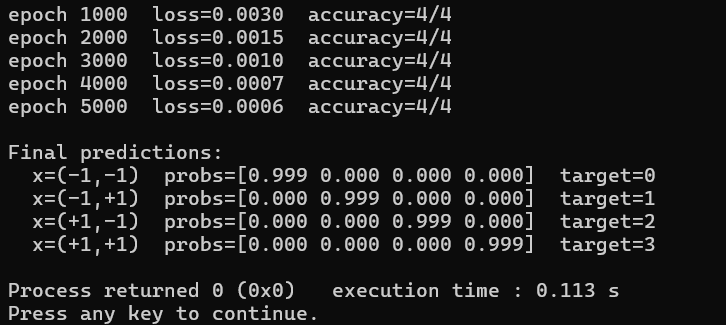
Figure 4-11 trains a four class network on the pair. Watch the loss decrease and accuracy reach 4/4. The softmax output gives you a probability distribution across all four classes. The cross-entropy loss drives the network to assign high probability to the correct class. The combined gradient (p - t) is simple and numerically stable.
4.11 When to Use What
MSE suits regression, meaning any problem where the answer is a continuous number such as a temperature, a price, a voltage or a sensor reading, and the output layer for it is a single neuron with either a linear activation or none at all.
Binary cross-entropy suits binary classification, meaning any problem whose answer is one of two labels such as yes against no or defective against good, and the output layer for it is a single neuron with a sigmoid activation whose value is read as the probability of the positive class.
Categorical cross-entropy with softmax suits multi-class classification, meaning digit recognition across ten classes, object detection across many, or next token prediction across a whole vocabulary, and the output layer for it carries one neuron per class where softmax turns the scores into probabilities and cross-entropy measures how far that distribution sits from the target.
For the rest of this book we use MSE when building up concepts (Chapters 5-6), BCE for binary classifiers, and softmax + cross-entropy for everything from CNNs onward. Transformers use cross-entropy over a vocabulary of thousands of tokens. The math is identical to what we built here, just with more classes.
4.12 Key Takeaways
A loss function scores how wrong the network is. Its derivative tells the network which direction to adjust.
MSE penalizes large errors quadratically. Good for regression but has vanishing gradient problems with sigmoid outputs in classification.
Binary cross-entropy pairs naturally with sigmoid. The gradient does not vanish when the prediction is confidently wrong.
Softmax converts a vector of raw logits into a probability distribution (non-negative, sums to 1). Subtract the max before computing exp to prevent overflow.
Categorical cross-entropy measures the distance between the predicted distribution and the target. Combined with softmax, the gradient simplifies to (prediction - target).
Numerical stability matters. Clamp values away from 0 before taking log. Subtract the max before taking exp. KANN uses 1e-9 as the safety floor.
4.13 Exercises
Compute MSE and BCE for the same set of predictions by hand. At what prediction value does BCE give a larger gradient than MSE?
Implement softmax for 10 classes and feed it logits where one class has value 1000 and all others have value 0. Verify the output is correct and does not overflow.
Modify 025_Train_Compare.c to use MSE instead of cross-entropy (use one-hot targets and MSE between probs and targets). Compare convergence speed. How many more epochs does MSE need?
Write a function that computes the softmax-crossentropy gradient numerically (perturb each logit by h = 0.0001, recompute loss, take the difference). Verify it matches (p - t) for each class.
What happens if you forget the numerical stability clamp and call logf(0.0f)? What does your system output? This is the kind of bug that crashes a training run at 3 AM.
Read the softmax implementation in KANN (kautodiff.c, search for kad_op_softmax). Compare the max-subtraction trick to yours. What does KANN do differently in the backward pass?